|
|
| (19 intermediate revisions by 2 users not shown) |
| Line 1: |
Line 1: |
| − | {{short description|Mapping that associates a single output value to each input}}
| + | ==Introduction== |
| − | {{redirect|f(x)|the girl group|f(x) (group)}}
| + | Formally, a function f from a set X to a set Y is defined by a set G of ordered pairs (x, y) such that x ∈ X, y ∈ Y, and every element of X is the first component of exactly one ordered pair in G. In other words, for every x in X, there is exactly one element y such that the ordered pair (x, y) belongs to the set of pairs defining the function f. The set G is called the graph of the function. Formally speaking, it may be identified with the function, but this hides the usual interpretation of a function as a process. Therefore, in common usage, the function is generally distinguished from its graph.}} |
| − | {{Functions}}
| + | Whenever one quantity uniquely determines the value of another quantity, we have a function. That is, the set <math>X</math> uniquely determines the set <math>Y</math>. You can think of a ''function'' as a kind of machine. You feed the machine raw materials, and the machine changes the raw materials into a finished product. |
| | | | |
| − | In [[mathematics]], a '''function'''<ref group=note>The words '''map''', '''mapping''', '''transformation''', '''correspondence''', and '''operator''' are often used synonymously. {{harvnb |Halmos |1970 |p=30}}.</ref> is a [[binary relation]] over two [[Set (mathematics)|sets]] that associates to every element of the first set ''exactly'' one element of the second set. Typical examples are functions from [[integer]]s to integers or from the [[real number]]s to real numbers.
| + | ===Functions in everyday life=== |
| | + | Think about dropping a ball from a bridge. At each moment in time, the ball is a height above the ground. The height of the ball is a function of time. It was the job of physicists to come up with a formula for this function. This type of function is called ''real-valued'' since the "finished product" is a number (or, more specifically, a real number). |
| | | | |
| − | Functions were originally the idealization of how a varying quantity depends on another quantity. For example, the position of a [[planet]] is a ''function'' of time. [[History of the function concept|Historically]], the concept was elaborated with the [[infinitesimal calculus]] at the end of the 17th century, and, until the 19th century, the functions that were considered were [[differentiable function|differentiable]] (that is, they had a high degree of regularity). The concept of function was formalized at the end of the 19th century in terms of [[set theory]], and this greatly enlarged the domains of application of the concept.
| + | Think about a wind storm. At different places, the wind can be blowing in different directions with different intensities. The direction and intensity of the wind can be thought of as a function of position. This is a function of two real variables (a location is described by two values - an <math>x</math> and a <math>y</math>) which results in a vector (which is something that can be used to hold a direction and an intensity). These functions are studied in multivariable calculus (which is usually studied after a one year college level calculus course). This a vector-valued function of two real variables. |
| | | | |
| − | A function is a process or a relation<!-- Please, do not link to [[Binary relation]], this is not the technical meaning that is intended--> that associates each element {{mvar|x}} of a [[set (mathematics)|set]] {{mvar|X}}, the ''[[domain of a function|domain]]'' of the function, to a single element {{mvar|y}} of another set {{mvar|Y}} (possibly the same set), the ''[[codomain]]'' of the function. If the function is called {{mvar|f}}, this relation is denoted {{math|1=''y'' = ''f''{{space|hair}}(''x'')}} (which is spoken aloud as {{mvar|f}} of {{mvar|x}}), the element {{mvar|x}} is the ''[[argument of a function|argument]]'' or ''input'' of the function, and {{mvar|y}} is the ''value of the function'', the ''output'', or the ''image'' of {{mvar|x}} by {{mvar|f}}.<ref name=MacLane>{{cite book | last = MacLane | first = Saunders | authorlink = Saunders MacLane | last2 = Birkhoff | first2 = Garrett | author2-link = Garrett Birkhoff | title = Algebra | url = https://archive.org/details/algebra00macl | url-access = registration | publisher = Macmillan | edition = First | year = 1967 | location = New York | pages = [https://archive.org/details/algebra00macl/page/1 1–13] }}</ref> The symbol that is used for representing the input is the [[variable (mathematics)|variable]] of the function (one often says that {{mvar|f}} is a function of the variable {{mvar|x}}).
| + | We will be looking at real-valued functions until studying multivariable calculus. Think of a real-valued function as an ''input-output machine''; you give the function an input, and it gives you an output which is a number (more specifically, a real number). For example, the squaring function takes the input 4 and gives the output value 16. The same squaring function takes the input -1 and gives the output value 1. |
| | + | [[File:Function machine2.svg|thumb|right|This is an intuitive way to understand functions: a machine that makes the input <math>x</math> go through a transformation <math>f</math> into the output <math>f(x)</math>]] |
| | | | |
| − | A function is uniquely represented by the set of all [[pair (mathematics)|pairs]] {{math|(''x'', ''f''{{space|hair}}(''x''))}}, called the [[graph of a function|graph]] of the function.<ref group=note>This definition of "graph" refers to a ''set'' of pairs of objects. Graphs, in the sense of ''diagrams'', are most applicable to functions from the real numbers to themselves. All functions can be described by sets of pairs but it may not be practical to construct a diagram for functions between other sets (such as sets of matrices).</ref> When the domain and the codomain are sets of real numbers, each such pair may be considered as the [[Cartesian coordinates]] of a point in the plane. The set of these points is called the graph of the function; it is a popular means to illustrate the function.
| + | === Notation === |
| | + | Functions are used so much that there is a special notation for them. The notation is somewhat ambiguous, so familiarity with it is important in order to understand the intention of an equation or formula. |
| | | | |
| − | Functions are widely used in [[science]], and in most fields of mathematics. It has been said that functions are "the central objects of investigation" in most fields of mathematics.{{sfn |Spivak |2008 |p=39}}
| + | Though there are no strict rules for naming a function, it is standard practice to use the letters <math>f</math> , <math>g</math> , and <math>h</math> to denote functions, and the variable <math>x</math> to denote an independent variable. <math>y</math> is used for both dependent and independent variables. |
| | | | |
| − | [[File:Function machine2.svg|thumb|right|Schematic depiction of a function described metaphorically as a "machine" or "[[black box]]" that for each input yields a corresponding output]]
| + | When discussing or working with a function <math>f</math> , it's important to know not only the function, but also its independent variable <math>x</math> . Thus, when referring to a function <math>f</math>, you usually do not write <math>f</math>, but instead <math>f(x)</math> . The function is now referred to as "<math>f</math> of <math>x</math>". The name of the function is adjacent to the independent variable (in parentheses). This is useful for indicating the value of the function at a particular value of the independent variable. For instance, if |
| − | [[Image:Graph of example function.svg|thumb|right|The red curve is the [[graph of a function]], because any [[Vertical line test|vertical line]] has exactly one crossing point with the curve.]]
| + | :<math>f(x)=7x+1</math> , |
| | + | and if we want to use the value of <math>f</math> for <math>x</math> equal to <math>2</math> , then we would substitute 2 for <math>x</math> on both sides of the definition above and write |
| | + | :<math>f(2)=7(2)+1=14+1=15</math> |
| | | | |
| − | [[File:Function color example 3.svg|thumb|A function that associates any of the four colored shapes to its color.]]
| + | This notation is more informative than leaving off the independent variable and writing simply '<math>f</math>' , but can be ambiguous since the parentheses next to <math>f</math> can be misinterpreted as multiplication, <math>2f</math>. To make sure nobody is too confused, follow this procedure: |
| | | | |
| − | ==Definition== | + | # Define the function <math>f</math> by equating it to some expression. |
| − | {{multiple image| width = 220
| + | # Give a sentence like the following: "At <math>x=c</math>, the function <math>f</math> is..." |
| − | | align = right
| + | # Evaluate the function. |
| − | | direction = vertical
| + | |
| − | | image1 = Injection keine Injektion 2a.svg
| + | === Description === |
| − | | caption1 = Diagram of a function, with domain ''X'' = {1, 2, 3} and codomain ''Y'' = {A, B, C, D}, which is defined by the set of ordered pairs {(1, D), (2, C), (3, C)}. The image/range is the set {C, D}.
| + | There are many ways which people describe functions. In the examples above, a verbal descriptions is given (the height of the ball above the earth as a function of time). Here is a list of ways to describe functions. The top three listed approaches to describing functions are the most popular. |
| − | <br /><hr style="height:8pt; visibility:hidden"> | + | |
| − | ----<hr style="height:8pt; visibility:hidden">
| + | # A function is given a name (such as <math>f</math>) and a formula for the function is also given. For example, <math>f(x)=3x+2</math> describes a function. We refer to the input as the '''argument''' of the function (or the '''independent variable'''), and to the output as the '''value''' of the function at the given argument. |
| − | |
| + | # A function is described using an equation and two variables. One variable is for the input of the function and one is for the output of the function. The variable for the input is called the '''independent variable'''. The variable for the output is called the '''dependent variable'''. For example, <math>y=3x+2</math> describes a function. The dependent variable appears by itself on the left hand side of equal sign. |
| − | | image2 = Injection keine Injektion 1.svg
| + | # A verbal description of the function. |
| − | | caption2 = This diagram, representing the set of pairs {(1,D), (2,B), (2,C)}, does ''not'' define a function. One reason is that 2 is the first element in more than one ordered pair, {{nowrap|(2, B)}} and {{nowrap|(2, C)}}, of this set. Two other reasons, also sufficient by themselves, is that neither 3 nor 4 are first elements (input) of any ordered pair therein.
| + | |
| − | }}
| + | When a function is given a name (like in number 1 above), the name of the function is usually a single letter of the alphabet (such as <math>f</math> or <math>g</math>). Some functions whose names are multiple letters (like the sine function <math>y=\sin(x)</math> |
| − | Intuitively, a function is a process that associates to each element of a set {{math|''X''}} a single element of a set {{math|''Y''}}.
| + | |
| | + | ===Plugging a value into a function=== |
| | + | If we write <math>f(x)=3x+2</math> , then we know that |
| | + | |
| | + | *The function <math>f</math> is a function of <math>x</math> . |
| | + | *To evaluate the function at a certain number, replace the <math>x</math> with that number. |
| | + | *Replacing <math>x</math> with that number in the right side of the function will produce the function's output for that certain input. |
| | + | *In English, the definition of <math>f</math> is interpreted, "Given a number, <math>f</math> will return ''two more than the triple of that number''." |
| | + | |
| | + | How would we know the value of the function <math>f</math> at 3? |
| | + | We would have the following three thoughts: |
| | + | |
| | + | # <math>f(3)=3(3)+2</math> |
| | + | # <math>3(3)+2=9+2</math> |
| | + | # <math>9+2=11</math> |
| | + | and we would write |
| | + | |
| | + | <math>f(3)=3(3)+2=9+2=11</math>. |
| | + | |
| | + | The value of <math>f</math> at 3 is 11. |
| | + | |
| | + | Note that <math>f(3)</math> means the value of the dependent variable when <math>x</math> takes on the value of 3. So we see that the number ''11'' is the output of the function when we give the number ''3'' as the input. People often summarize the work above by writing "the value of <math>f</math> at three is eleven", or simply "<math>f</math> of three equals eleven". |
| | + | |
| | + | ==Basic concepts of functions== |
| | + | The formal definition of a function states that a function is actually a ''mapping'' that associates the elements of one set called the '''domain''' of the function, <math>A</math>, with the elements of another set called the ''range'' of the function, <math>B</math>. For each value we select from the domain of the function, there exists ''exactly one'' corresponding element in the range of the function. The definition of the function tells us which element in the range corresponds to the element we picked from the domain. An example of how is given below. |
| | + | |
| | + | ===Example=== |
| | + | Let function <math>f(x)=5x+\frac{5x}{2}</math> for all <math>x</math>. For what value of <math>x</math> gives <math>f(x)=225\frac{1}{2}</math> |
| | + | In mathematics, it is important to notice any repetition. If something seems to repeat, keep a note of that in the back of your mind somewhere. |
| | | | |
| − | Formally, a function {{math|''f''}} from a set {{math|''X''}} to a set {{math|''Y''}} is defined by a set {{mvar|G}} of ordered pairs {{math|(''x'', ''y'')}} such that {{math|''x'' ∈ ''X''}}, {{math|''y'' ∈ ''Y''}}, and every element of {{math|''X''}} is the first component of exactly one ordered pair in {{mvar|G}}.<ref>{{cite book |last=Hamilton |first=A. G. |title=Numbers, sets, and axioms: the apparatus of mathematics |page=[https://archive.org/details/numberssetsaxiom0000hami/page/83 83] |publisher=Cambridge University Press |isbn=978-0-521-24509-8 |url=https://archive.org/details/numberssetsaxiom0000hami|url-access=registration |quote=function is a relation. |year=1982 }}</ref><ref group="note">The sets ''X'', ''Y'' are parts of data defining a function; i.e., a function is a set of ordered pairs <math>(x, y)</math> with <math>x \in X, y \in Y</math>, together with the sets ''X'', ''Y'', such that for each <math>x \in X</math>, there is a unique <math>y \in Y</math> with <math>(x, y)</math> in the set.</ref> In other words, for every {{math|''x''}} in {{math|''X''}}, there is exactly one element {{math|''y''}} such that the ordered pair {{math|(''x'', ''y'')}} belongs to the set of pairs defining the function {{math|''f''}}. The set {{mvar|G}} is called the [[graph of a function|graph of the function]]. Formally speaking, it may be identified with the function, but this hides the usual interpretation of a function as a process. Therefore, in common usage, the function is generally distinguished from its graph. Functions are also called ''[[Map (mathematics)|maps]]'' or ''mappings'', though some authors make some distinction between "maps" and "functions" (see section [[#Map]]).
| + | Here, notice that <math>f(x)=5x+\frac{5x}{2}</math> and <math>f(x)=225\frac{1}{2}</math>. Because <math>f(x)</math> is equal to two different things, it must be the case that the other side of the equal sign to <math>f(x)</math> is equal to the other. This property is known as the transitive property and could thus make the following equation below true:<br> |
| | + | :<math>225\frac{1}{2}=5x+\frac{5x}{2}</math> |
| | | | |
| − | In the definition of function, {{math|''X''}} and {{math|''Y''}} are respectively called the ''domain'' and the ''codomain'' of the function {{mvar|f}}. If {{math|(''x'', ''y'')}} belongs to the set defining {{mvar|f}}, then {{mvar|y}} is the ''image'' of {{mvar|x}} under {{mvar|f}}, or the ''value'' of {{mvar|f}} applied to the ''argument'' {{mvar|x}}. Especially in the context of numbers, one says also that {{mvar|y}} is the value of {{mvar|f}} for the ''value {{mvar|x}} of its variable'', or, still shorter, {{mvar|y}} is the ''value of'' {{mvar|f}} ''of'' {{mvar|x}}, denoted as {{math|''y'' {{=}} ''f''(''x'')}}. | + | Next, simplify — make your life easier rather than harder. In this instance, since <math>5x+\frac{5x}{2}</math> has <math>x</math> as a like-term, and the two terms are fractions added to the other, put it over a common denominator and simplify. Similar, since <math>225\frac{1}{2}</math> is a mixed fraction, <math>225\frac{1}{2}=225+\frac{1}{2}</math>.<br> |
| | + | :<math>225\frac{1}{2}=5x+\frac{5x}{2}</math><br> |
| | + | :<math>\Rightarrow\frac{225}{1}+\frac{1}{2}=\frac{5x}{1}+\frac{5x}{2}</math><br> |
| | + | :<math>\Rightarrow\frac{450}{2}+\frac{1}{2}=\frac{10x}{2}+\frac{5x}{2}</math><br> |
| | + | :<math>\Rightarrow\frac{451}{2}=\frac{15x}{2}</math> |
| | | | |
| − | Two functions {{mvar|f}} and {{mvar|g}} are equal if their domain and codomain sets are the same and their output values agree on the whole domain. Formally, {{math|1=''f'' = ''g''}} if {{math|1=''f''(''x'') = ''g''(''x'')}} for all {{math|''x'' ∈ ''X''}}, where {{math|''f'':''X'' → ''Y''}} and {{math|''g'':''X'' → ''Y''}}.{{sfn |Apostol |1981 |p=35}}{{sfn |Kaplan |1972 |p=25}}<ref group=note>This follows from the [[axiom of extensionality]], which says two sets are the same if and only if they have the same members. Some authors drop codomain from a definition of a function, and in that definition, the notion of equality has to be handled with care; see, for example, {{cite web |url=https://math.stackexchange.com/q/1403122 |date=August 19, 2015 |title=When do two functions become equal? |work=[[Stack Exchange]] }}</ref>
| + | Multiply both sides by the reciprocal of the coefficient of <math>x</math>, <math>\frac{2}{15}</math> from both sides by multiplying by it.<br> |
| | + | :<math>\frac{2}{15}\cdot\frac{451}{2}=x</math><br> |
| | + | :<math>\frac{451}{15}=x</math> ''or'' <math>x=\frac{451}{15}</math>. |
| | | | |
| − | The domain and codomain are not always explicitly given when a function is defined, and, without some (possibly difficult) computation, one knows only that the domain is contained in a larger set. Typically, this occurs in [[mathematical analysis]], where "a function {{nowrap|from {{mvar|X}} to {{mvar|Y}} "}} often refers to a function that may have a proper subset<ref group=note>called the ''domain of definition'' by some authors, notably computer science</ref> of {{mvar|X}} as domain. For example, a "function from the reals to the reals" may refer to a [[real-valued function|real-valued]] function of a [[function of a real variable|real variable]], and this phrase does not mean that the domain of the function is the whole set of the [[real number]]s, but only that the domain is a set of real numbers that contains a non-empty [[open interval]]; such a function is then called a [[partial function]]. For example, if {{mvar|f}} is a function that has the real numbers as domain and codomain, then a function mapping the value {{mvar|x}} to the value <math>g(x)=\tfrac 1{f(x)}</math> is a function {{mvar|g}} from the reals to the reals, whose domain is the set of the reals {{mvar|x}}, such that {{math|''f''(''x'') ≠ 0}}. | + | The value of <math>x</math> that makes <math>f(x)=225\frac{1}{2}</math> is <math>x=\frac{451}{15}</math>. |
| | | | |
| − | The [[range of a function|range]] of a function is the set of the images of all elements in the domain. However, ''range'' is sometimes used as a synonym of codomain, generally in old textbooks.{{citation needed|reason=Give an example reference for both meanings, also to illustrate what 'old' refers to (this changes over time).|date=March 2019}}
| + | Classically, the element picked from the domain is pictured as something that is fed into the function and the corresponding element in the range is pictured as the output. Since we "pick" the element in the domain whose corresponding element in the range we want to find, we have control over what element we pick and hence this element is also known as the "independent variable". The element mapped in the range is beyond our control and is "mapped to" by the function. This element is hence also known as the "dependent variable", for it depends on which independent variable we pick. Since the elementary idea of functions is better understood from the classical viewpoint, we shall use it hereafter. However, it is still important to remember the correct definition of functions at all times. |
| | | | |
| − | ===Relational approach=== | + | === Basic types of transformation === |
| − | Any subset of the Cartesian product of two sets <math>X</math> and <math>Y</math> defines a [[binary relation]] <math>R\subseteq X \times Y</math> between these two sets. It is immediate that an arbitrary relation may contain pairs that violate the necessary conditions for a function, given above.
| + | To make it simple, for the function <math>f(x)</math>, all of the possible <math>x</math> values constitute the domain, and all of the values <math>f(x)</math> (<math>y</math> on the x-y plane) constitute the range. To put it in more formal terms, a function <math>f</math> is a mapping of some element <math>a\in A</math>, called the domain, to exactly one element <math>b\in B</math>, called the range, such that <math>f:A\to B</math>. The image below should help explain the modern definition of a function: |
| | + | [[File:Function_Definition.svg|alt=The image demonstrates a mapping of some element a (the circle) in A, the domain, to exactly one element b in B, the range.|thumb|<math>A</math> is the domain of the function while <math>B</math> is the range. This transformation from set <math>A</math> to <math>B</math> is an example of one-to-one function.]] |
| | + | # A function is considered '''one-to-one''' if an element <math>a\in A</math> from domain <math>A</math> of function <math>f</math>, leads to exactly one element <math>b\in B</math> from range <math>B</math> of the function. By definition, since only one element <math>b</math> is mapped by function <math>f</math> from some element <math>a</math>, <math>f:A\to B</math> implies that there exists only one element <math>b</math> from the mapping. Therefore, there exists a one-to-one function because it complies with the definition of a function. This definition is similar to '''''Figure 1'''''. |
| | + | # A function is considered '''many-to-one''' if some elements <math>a_{1},a_{2},\ldots a_{n}\in A</math> from domain <math>A</math> of function <math>f</math> maps to exactly one element <math>b\in B</math> from range <math>B</math> of the function. Since some elements <math>\left( a_{1},a_{2},\ldots a_{n} \right)\in A</math> must map onto exactly one element <math>b\in B</math>, <math>f:A\to B</math> must be compliant with the definition of a function. Therefore, there exists a many-to-one function. |
| | + | # A function is considered '''one-to-many''' if exactly one element <math>a\in A</math> from domain <math>A</math> of function <math>f</math> maps to some elements <math>\left( b_{1},b_{2},\ldots b_{n} \right)\in B</math> from range <math>B</math> of the function. If some element <math>a</math> maps onto many distinct elements <math>b</math>, then <math>f:A\to B</math> is non-functional since there exists many distinct elements <math>b</math>. Given many-to-one is non-compliant to the definition of a function, there exists no function that is one-to-many. |
| | | | |
| − | A binary relation is [[Functional relation|functional]] (also called right-unique) if
| + | The modern definition describes a function sufficiently such that it helps us determine whether some new type of "function" is indeed one. Now that each case is defined above, you can now prove whether functions are one of these function cases. Here is an example problem: |
| − | : <math>\forall x \in X, \forall y \in Y, \forall z \in Y, (x, y) \in R \land (x, z) \in R \implies y = z.</math>
| |
| | | | |
| − | A binary relation is [[Serial relation|serial]] (also called left-total) if
| + | ===One-to-One Example=== |
| − | : <math>\forall x \in X, \exists y \in Y, (x, y) \in R.</math> | + | '''Given''': <math>f(x)=ax+b</math>, where <math>a</math> and <math>b</math> are constant and <math>a\ne0</math>.<br> |
| | + | '''Prove''': function <math>f</math> is one-to-one.}} Notice that the only changing element in the function <math>f</math> is <math>x</math>. To prove a function is one-to-one by applying the definition may be impossible because although two random elements of domain set <math>A</math> may not be many-to-one, there may be some elements <math>\left( a_{1},a_{2},\ldots a_{n} \right)\in A</math> that may make the function many-to-one. To account for this possibility, we must prove that it is impossible to have some result like that. |
| | | | |
| − | A [[partial function]] is a binary relation that is functional.
| + | Assume there exists two distinct elements <math>x_{1}\ne x_2</math> that will result in <math>f\left( x_{1} \right) =f\left( x_{2} \right)</math>. This would make the function many-to-one. In consequence,<br> |
| | + | <math display="block">ax_{1}+b=ax_{2}+b</math> |
| | | | |
| − | A function is a binary relation that is functional and serial.
| + | Subtract <math>b</math> from both sides of the equation. |
| | + | :<math>\Rightarrow ax_{1}=ax_{2}</math> |
| | | | |
| − | Various properties of functions and function composition may be reformulated in the language of relations. For example, a function is [[injective function|injective]] if the [[converse relation]] <math>R^{\text{T}}\subseteq Y \times X</math> is functional, where the converse relation is defined as <math>R^{\text{T}} = \{(y,x) \mid (x,y) \in R\}.</math><ref name=RM>[[Gunther Schmidt]]( 2011) ''Relational Mathematics'', Encyclopedia of Mathematics and its Applications, vol. 132, sect 5.1 Functions, pp. 49–60, [[Cambridge University Press]] {{ISBN|978-0-521-76268-7}} [http://www.cambridge.org/us/academic/subjects/mathematics/logic-categories-and-sets/relational-mathematics?format=HB CUP blurb for ''Relational Mathematics'']</ref>
| + | Subtract <math>ax_{2}</math> from both sides of the equation. |
| | + | :<math>\Rightarrow ax_{1}-ax_{2}=0</math> |
| | | | |
| − | ===As an element of a Cartesian product over a domain ===
| + | Factor <math>a</math> from both terms to the left of the equation. |
| − | The set of all functions from some given domain to a codomain is sometimes identified with the Cartesian product of copies of the codomain, [[index set|indexed]] by the domain. Namely, given sets <math>X</math> and <math>Y,</math> any function <math>f\colon X \to Y</math> is an element of the Cartesian product of copies of <math>Y</math>s over the index set <math>X</math>
| + | :<math>\Rightarrow a\left( x_{1}-x_{2} \right) =0</math> |
| − | :<math>f \in \prod_X Y = Y^X.</math> | |
| | | | |
| − | Viewing <math>f</math> as [[tuple]] with coordinates, then for each <math>x \in X</math>, the <math>x</math>th coordinate of this tuple is the value <math>f(x) \in Y.</math> This reflects the intuition that for each <math>x \in X,</math> the function ''picks'' some element <math>y \in Y,</math> namely, <math>f(x).</math> (This point of view is used for example in the discussion of a [[choice function]].)
| + | Multiply <math>\frac{1}{a}</math> to both sides of the equation. |
| | + | :<math>\Rightarrow \left( x_{1}-x_{2} \right) =0</math> |
| | | | |
| − | Infinite Cartesian products are often simply "defined" as sets of functions.<ref>Halmos, Naive Set Theory, 1968, sect.9 ("Families")</ref>
| + | Add <math>x_{2}</math> to both sides of the equation. |
| | + | :<math>\Rightarrow x_{1}=x_{2}</math> |
| | | | |
| − | ==Notation== | + | Notice that <math>x_{1}=x_{2}</math>. However, this is impossible because <math>x_{1}</math> and <math>x_{2}</math> are distinct. Ergo, <math>f\left( x_{1} \right)\ne f\left( x_{2} \right)</math>. No two distinct inputs can give the same output. Therefore, the function must be one-to-one. |
| | | | |
| − | There are various standard ways for denoting functions. The most commonly used notation is functional notation, which defines the function using an equation that gives the names of the function and the argument explicitly. This gives rise to a subtle point, often glossed over in elementary treatments of functions: ''functions'' are distinct from their ''values''. Thus, a function {{math|''f''}} should be distinguished from its value {{math|''f''(''x''<sub>0</sub>)}} at the value {{math|''x''<sub>0</sub>}} in its domain. To some extent, even working mathematicians will conflate the two in informal settings for convenience, and to avoid appearing pedantic. However, strictly speaking, it is an [[abuse of notation]] to write "let <math>f\colon \mathbb{R}\to\mathbb{R}</math> be the function {{math|1=''f''(''x'') = ''x''<sup>2</sup>}} ", since {{math|''f''(''x'')}} and {{math|''x''<sup>2</sup>}} should both be understood as the ''value'' of ''f'' at ''x'', rather than the function itself. Instead, it is correct, though long-winded, to write "let <math>f\colon \mathbb{R}\to\mathbb{R}</math> be the function defined by the equation {{math|1=''f''(''x'') = ''x''<sup>2</sup>,}} valid for all real values of {{math|''x''}} ". A compact phrasing is "let <math>f\colon \mathbb{R}\to\mathbb{R}</math> with {{math|1=''f''(''x'') = ''x''<sup>2</sup>,}}" where the redundant "be the function" is omitted and, by convention, "for all <math>x</math> in the domain of <math>f</math>" is understood.
| + | === Basic concepts === |
| | + | [[File:Domain, Range, Codomain.svg|thumb|230x230px|The domain is all the elements in set <math>A</math> that can be mapped to the elements in set <math>B</math>. |
| | | | |
| − | This distinction in language and notation becomes important in cases where functions themselves serve as inputs for other functions. (A function taking another function as an input is termed a ''[[Functional (mathematics)|functional]]''.) Other approaches to denoting functions, detailed below, avoid this problem but are less commonly used.
| + | The range is those elements in set <math>B</math> which are mapped with the domain. |
| | | | |
| − | ===Functional notation===
| + | The codomain is all the elements in set <math>B</math>.]]There are a few more important ideas to learn from the modern definition of the function, and it comes from knowing the difference between domain, range, and codomain. We already discussed some of these, yet knowing about sets adds a new definition for each of the following ideas. Therefore, let us discuss these based on these new ideas. Let <math>A</math> and <math>B</math> be a set. If we were to combine these two sets, it would be defined as the ''cartesian cross product'' <math>A\times B</math>. The subset of this product is the function. The below definitions are a little confusing. The best way to interpret these is to draw an image. To the right of these definitions is the image that corresponds to it. |
| − | As first used by [[Leonhard Euler]] in 1734,<ref>{{citation |page=19 |title=Calculus of a Single Variable |author=Ron Larson, Bruce H. Edwards |publisher=Cengage Learning |year=2010 |isbn=978-0-538-73552-0}}</ref> functions are denoted by a symbol consisting generally of a single letter in [[italic font]], most often the lower-case letters {{math|''f'', ''g'', ''h''}}. Some widely used functions are represented by a symbol consisting of several letters (usually two or three, generally an abbreviation of their name). By convention, in this case, a [[roman type]] is used, such as "{{math|sin}}" for the [[sine function]], in contrast to italic font for single-letter symbols.
| |
| | | | |
| − | The notation (read: "{{mvar|y}} equals {{mvar|f}} of {{mvar|x}}")
| + | ====Definition of domain, range, and codomain of a function==== |
| − | :<math>y=f(x)</math>
| |
| − | means that the pair {{math|(''x'', ''y'')}} belongs to the set of pairs defining the function {{mvar|f}}. If {{mvar|X}} is the domain of {{mvar|f}}, the set of pairs defining the function is thus, using [[set-builder notation]],
| |
| − | :<math>\{(x, f(x)) : x\in X\}.</math>
| |
| | | | |
| − | Often, a definition of the function is given by what ''f'' does to the explicit argument ''x.'' For example, a function ''f'' can be defined by the equation
| + | The '''domain''' is defined to be a set <math>A</math> |
| | + | with all elements <math>a\in A</math> mapping to at least one unique <math>b\in B</math> . |
| | | | |
| − | :<math>f(x)=\sin(x^2+1)</math> | + | The set of elements in <math>B</math> is the '''range''' of the function mapping <math>f:A\to B</math> in the cartesian cross product, whereby the set of all elements <math>a\in A</math> maps to some element <math>b\in B</math> . |
| | | | |
| − | for all real numbers ''x.'' In this example, ''f'' can be thought of as the [[#Function composition|composite]] of several simpler functions: squaring, adding 1, and taking the sine. However, only the sine function has a common explicit symbol (sin), while the combination of squaring and then adding 1 is described by the polynomial expression <math>x^2+1</math>. In order to explicitly reference functions such as squaring or adding 1 without introducing new function names (e.g., by defining function ''g'' and ''h'' by <math>g(x)=x^2</math> and <math>h(x)=x+1</math>), one of the methods below (arrow notation or dot notation) could be used.
| + | The '''codomain''' is the set <math>B</math>, where it is not necessarily the case that all elements <math>b\in B</math> was mapped by some <math>a\in A</math>. |
| | | | |
| − | Sometimes the parentheses of functional notation are omitted when the symbol denoting the function consists of several characters and no ambiguity may arise. For example, <math>\sin x</math> can be written instead of <math>\sin(x).</math>
| + | Note that the codomain is not as important as the other two concepts. |
| | | | |
| − | ===Arrow notation=== | + | Take <math>f(x)=\sqrt{1-x^2}</math> for example:[[Image:Domainofsemicirclefunction.png|thumb|The domain of the function is the interval from -1 to 1]]Because of the square root, the content in the square root should be strictly not smaller than 0.<blockquote><math>1-x^2\geq0</math></blockquote><blockquote><math>\Leftrightarrow -1\leq x\leq 1</math></blockquote>Thus the domain is<blockquote><math>x\in[-1,1]</math></blockquote>[[Image:Rangeofsemicirclefunction.png|thumb|The range of the function is the interval from 0 to 1]] |
| − | For explicitly expressing domain {{math|''X''}} and the codomain {{math|''Y''}} of a function {{math|''f''}}, the arrow notation is often used (read: {{nowrap|"the function {{math|''f''}} from {{mvar|X}} to {{mvar|Y}}"}} or {{nowrap|"the function {{math|''f''}} mapping elements of {{mvar|X}} to elements of {{mvar|Y}}"}}):
| |
| | | | |
| − | :<math>f\colon X \to Y</math>
| + | Correspondingly, the range will be<blockquote><math>f(x)\in[0,1]</math></blockquote> |
| − | or
| |
| − | :<math>X ~ \stackrel{f}{\to} ~ Y.</math>
| |
| | | | |
| − | This is often used in relation with the arrow notation for elements (read: "{{mvar|f}} maps {{mvar|x}} to {{math|''f''{{space|hair}}(''x'')}}"), often stacked immediately below the arrow notation giving the function symbol, domain, and codomain:
| + | === Other types of transformation === |
| − | :<math>x\mapsto f(x).</math>
| + | There is one more final aspect that needs to be defined. We already have a good idea of what makes a mapping a function (e.g. it cannot be one-to-many). However, three more definitions that you will often hear will be necessary to talk about: ''injective'', ''surjective'', ''bijective''. |
| | + | [[File:Injective, Surjective, Bijective.svg|488x488px|alt=|none|thumb|The function mapping on the left is an example of an injective function because it is one-to-one. However, it is not surjective because the range and the codomain are not the same.]] |
| | | | |
| − | For example, if a multiplication is defined on a set {{mvar|X}}, then the [[square function]] <math>\operatorname{sqr}</math> on {{mvar|X}} is unambiguously defined by (read: "the function <math>\operatorname{sqr}</math> from {{mvar|X}} to {{mvar|X}} that maps {{mvar|x}} to {{math|''x'' ⋅ ''x''}}")
| + | * A function is '''injective''' if it is one-to-one. |
| − | :<math>\begin{align}
| + | * A function is '''surjective''' if it is "onto." That is, the mapping <math>f:A\to B</math> has <math>B</math> as the ''range'' of the function, where the codomain and the range of the function are the same. |
| − | \operatorname{sqr}\colon X &\to X\\
| + | * A function is '''bijective''' if it is both surjective and injective. |
| − | x &\mapsto x\cdot x,\end{align}</math>
| |
| | | | |
| − | the latter line being more commonly written | + | Again, the above definitions are often very confusing. Again, another image is provided to the right of the bullet points. Along with that, another example is also provided. Let us analyze the function <math>g(x)=ax^{2}</math>. |
| − | :<math>x\mapsto x^2.</math>
| |
| | | | |
| − | Often, the expression giving the function symbol, domain and codomain is omitted. Thus, the arrow notation is useful for avoiding introducing a symbol for a function that is defined, as it is often the case, by a formula expressing the value of the function in terms of its argument. As a common application of the arrow notation, suppose <math>f\colon X\times X\to Y;\;(x,t) \mapsto f(x,t)</math> is a two-argument function, and we want to refer to a [[Partial application|partially applied function]] <math>X\to Y</math> produced by fixing the second argument to the value {{math|''t''<sub>0</sub>}} without introducing a new function name. The map in question could be denoted <math>x\mapsto f(x,t_0)</math> using the arrow notation for elements. The expression <math>x\mapsto f(x,t_0)</math> (read: "the map taking {{math|''x''}} to <math>f(x,t_0)</math>") represents this new function with just one argument, whereas the expression <math>f(x_0,t_0)</math> refers to the value of the function {{math|''f''}} at the {{nowrap|point <math>(x_0,t_0)</math>.}}
| + | '''Given''': <math>g(x)=ax^{2}</math>, where <math>a</math> is constant and <math>a\ne0</math>.<br> |
| | + | '''Prove''': function <math>g</math> is non-surjective and non-injective. |
| | | | |
| − | ===Index notation===
| + | Notice that the only changing element in the function <math>g</math> is <math>x</math>. Let us check to see the conditions of this function. |
| | | | |
| − | Index notation is often used instead of functional notation. That is, instead of writing {{math|''f''{{space|hair}}(''x'')}}, one writes <math>f_x.</math>
| + | '''Is it injective'''? Let <math>g(x)=y</math>, and solve for <math>x</math>. First, divide by <math>a</math>. |
| | + | :<math>y=ax^{2}</math> |
| | + | :<math>\Rightarrow \frac{y}{a}=x^{2}</math> |
| | | | |
| − | This is typically the case for functions whose domain is the set of the [[natural number]]s. Such a function is called a [[sequence (mathematics)|sequence]], and, in this case the element <math>f_n</math> is called the {{mvar|n}}th element of sequence.
| + | Then take the square root of <math>x^2</math>. By definition, <math>\sqrt{x^{2}}=\pm\sqrt{x^{2}}=\pm x</math>, so |
| | + | :<math>\frac{y}{a}=x^{2}</math> |
| | + | :<math>\Rightarrow\pm\sqrt{\frac{y}{a}}=\pm x</math> |
| | | | |
| − | The index notation is also often used for distinguishing some variables called [[parameter]]s from the "true variables". In fact, parameters are specific variables that are considered as being fixed during the study of a problem. For example, the map <math>x\mapsto f(x,t)</math> (see above) would be denoted <math>f_t</math> using index notation, if we define the collection of maps <math>f_t</math> by the formula <math>f_t(x)=f(x,t)</math> for all <math>x,t\in X</math>.
| + | Notice, however, what we learned from the above manipulation. As a result of solving for <math>x</math>, we found that there are two solutions for <math>x</math>. However, this resulted in two different values from <math>\frac{y}{a}</math>. This means that for some individual <math>x</math> that gives <math>y</math>, there are two different inputs that result in the same value. Because <math>f(x_{1})=f(x_{2})</math> when <math>x_{1}\ne x_{2}</math>, this is by definition non-injective. |
| | | | |
| − | ===Dot notation=== | + | '''Is it surjective'''? As a natural consequence of what we learned about inputs, let us determine the range of the function. After all, the only way to determine if something is surjective is to see if the range applies to all real numbers. A good way to determine this is by finding a pattern involving our domains. Let us say we input a negative number for the domain: <math>f(-x)=a(-x)^{2}=a\cdot(-x)\cdot(-x)=ax^2</math>. This seemingly trivial exercise tells us that negative numbers give us non-negative numbers for our range. This is huge information! For <math>x\in\mathbb{R}</math>, the function always results <math>y>0</math> for our range. For the set <math>B</math>, we have elements in that set that have no mappings from the set <math>A</math>. As such, <math>y\le0</math> is the codomain of set <math>B</math>. Therefore, this function is non-surjective! |
| | + | [[Image:Vertlinetest.png|thumb|This is an example of an expression which fails the vertical line test.]] |
| | | | |
| − | In the notation
| + | === Tests for equations === |
| − | <math>x\mapsto f(x),</math>
| |
| − | the symbol {{mvar|x}} does not represent any value, it is simply a [[placeholder name|placeholder]] meaning that, if {{mvar|x}} is replaced by any value on the left of the arrow, it should be replaced by the same value on the right of the arrow. Therefore, {{mvar|x}} may be replaced by any symbol, often an [[interpunct]] "{{math| ⋅ }}". This may be useful for distinguishing the function {{math|''f''{{space|hair}}(⋅)}} from its value {{math|''f''{{space|hair}}(''x'')}} at {{mvar|x}}.
| |
| | | | |
| − | For example, <math> a(\cdot)^2</math> may stand for the function <math> x\mapsto ax^2</math>, and <math>\textstyle \int_a^{\, (\cdot)} f(u)\,du</math> may stand for a function defined by an integral with variable upper bound: <math>\textstyle x\mapsto \int_a^x f(u)\,du</math>.
| + | ====The vertical line test==== |
| | + | The vertical line test is a systematic test to find out if an equation involving <math>x</math> and <math>y</math> can serve as a function (with <math>x</math> the independent variable and <math>y</math> the dependent variable). Simply graph the equation and draw a vertical line through each point of the <math>x</math>-axis. If any vertical line ever touches the graph at more than one point, then the equation is not a function; if the line always touches at most one point of the graph, then the equation is a function. |
| | | | |
| − | === Specialized notations ===
| + | The circle, on the right, is not a function because the vertical line intercepts two points on the graph when <math>x=1</math>. |
| − | There are other, specialized notations for functions in sub-disciplines of mathematics. For example, in [[linear algebra]] and [[functional analysis]], [[linear form]]s and the [[Vector (mathematics and physics)|vectors]] they act upon are denoted using a [[dual pair]] to show the underlying [[Duality (mathematics)|duality]]. This is similar to the use of [[bra–ket notation]] in quantum mechanics. In [[Mathematical logic|logic]] and the [[theory of computation]], the function notation of [[lambda calculus]] is used to explicitly express the basic notions of function [[Abstraction (computer science)|abstraction]] and [[Function application|application]]. In [[category theory]] and [[homological algebra]], networks of functions are described in terms of how they and their compositions [[Commutative property|commute]] with each other using [[commutative diagram]]s that extend and generalize the arrow notation for functions described above.
| |
| | | | |
| − | == Other terms == | + | ==== The horizontal line and the algebraic 1-1 test ==== |
| − | {| class="wikitable floatright" style= "width: 50%"
| + | Similarly, the horizontal line test, though does not test if an equation is a function, tests if a function is injective (one-to-one). If any horizontal line ever touches the graph at more than one point, then the function is not one-to-one; if the line always touches at most one point on the graph, then the function is one-to-one. |
| − | !Term
| |
| − | !Distinction from "function"
| |
| − | |-
| |
| − | | rowspan="3" |[[Map (mathematics)|Map/Mapping]]
| |
| − | |None; the terms are synonymous.<ref>{{Cite web|url=http://mathworld.wolfram.com/Map.html|title=Map|last=Weisstein|first=Eric W.|website=mathworld.wolfram.com|language=en|access-date=2019-06-12}}</ref>
| |
| − | |-
| |
| − | |A map can have ''any set'' as its codomain, while, in some contexts, typically in older books, the codomain of a function is specifically the set of [[real number|real]] or [[complex number|complex]] numbers.<ref>{{citation|last=Lang|first=Serge|title=Linear Algebra|page=83|year=1971|edition=2nd|publisher=Addison-Wesley}}</ref>
| |
| − | |-
| |
| − | |Alternatively, a map is associated with a ''special structure'' (e.g. by explicitly specifying a structured codomain in its definition). For example, a [[linear map]].<ref>{{cite book|title=Mathematical Analysis|author=T. M. Apostol|publisher=Addison-Wesley|year=1981|page=35}}</ref>
| |
| − | |-
| |
| − | |[[Homomorphism]]
| |
| − | |A function between two [[structure (mathematics)|structures]] of the same type that preserves the operations of the structure (e.g. a [[group homomorphism]]).<ref name=":0">{{Cite web|url=https://ncatlab.org/nlab/show/function|title=function in nLab|website=ncatlab.org|access-date=2019-06-12}}</ref><ref>{{Cite web|url=https://ncatlab.org/nlab/show/homomorphism|title=homomorphism in nLab|website=ncatlab.org|access-date=2019-06-12}}</ref>
| |
| − | |-
| |
| − | |[[Morphism]]
| |
| − | |A generalisation of homomorphisms to any [[Category (mathematics)|category]], even when the objects of the category are not sets (for example, a [[group (mathematics)|group]] defines a category with only one object, which has the elements of the group as morphisms; see {{slink|Category (mathematics)|Examples}} for this example and other similar ones).<ref>{{cite web|url=https://ncatlab.org/nlab/show/morphism|title=morphism|publisher=nLab|access-date=2019-06-12}}</ref><ref name=":0" /><ref>{{Cite web|url=http://mathworld.wolfram.com/Morphism.html|title=Morphism|last=Weisstein|first=Eric W.|website=mathworld.wolfram.com|language=en|access-date=2019-06-12}}</ref>
| |
| − | |}
| |
| | | | |
| − | ===Map===
| + | The algebraic 1-1 test is the non-geometric way to see if a function is one-to-one. The basic concept is that: |
| − | A function is often also called a '''map''' or a '''mapping''', but some authors make a distinction between the term "map" and "function". For example, the term "map" is often reserved for a "function" with some sort of special structure (e.g. [[maps of manifolds]]). In particular ''map'' is often used in place of ''homomorphism'' for the sake of succinctness (e.g., [[linear map]] or ''map from {{mvar|G}} to {{mvar|H}}'' instead of ''[[group homomorphism]] from {{mvar|G}} to {{mvar|H}}''). Some authors<ref>{{cite book|author=T. M. Apostol|title=Mathematical Analysis|year=1981|publisher=Addison-Wesley|page=35}}</ref> reserve the word ''mapping'' for the case where the structure of the codomain belongs explicitly to the definition of the function.
| |
| | | | |
| − | Some authors, such as [[Serge Lang]],<ref>{{citation|first=Serge|last=Lang|title=Linear Algebra|edition=2nd|year=1971|page=83|publisher=Addison-Wesley}}</ref> use "function" only to refer to maps for which the [[codomain]] is a subset of the [[real number|real]] or [[complex number|complex]] numbers, and use the term ''mapping'' for more general functions.
| + | Assume there is a function <math>f</math>. If:<blockquote><math>f(a)=f(b)</math>, and <math>a=b</math>, then</blockquote>function <math>f</math> is one-to-one. |
| | | | |
| − | In the theory of [[dynamical system]]s, a map denotes an [[Discrete-time dynamical system|evolution function]] used to create [[Dynamical system#Maps|discrete dynamical systems]]. See also [[Poincaré map]].
| + | Here is an example: prove that <math>f(x)=\frac{1-2x}{1+x}</math> is injective. |
| | | | |
| − | Whichever definition of ''map'' is used, related terms like ''[[Domain of a function|domain]]'', ''[[codomain]]'', ''[[Injective function|injective]]'', ''[[Continuous function|continuous]]'' have the same meaning as for a function.
| + | Since the notation is the notation for a function, the equation is a function. So we only need to prove that it is injective. Let <math>a</math> and <math>b</math> be the inputs of the function and that <math>f(a)=f(b)</math>. Thus, |
| | | | |
| − | ==Specifying a function==
| + | :<math>\frac{1-2a}{1+a}=\frac{1-2b}{1+b}</math> |
| − | Given a function <math>f</math>, by definition, to each element <math>x</math> of the domain of the function <math>f</math>, there is a unique element associated to it, the value <math>f(x)</math> of <math>f</math> at <math>x</math>. There are several ways to specify or describe how <math>x</math> is related to <math>f(x)</math>, both explicitly and implicitly. Sometimes, a theorem or an [[axiom]] asserts the existence of a function having some properties, without describing it more precisely. Often, the specification or description is referred to as the definition of the function <math>f</math>.
| + | :<math>\Leftrightarrow(1+b)(1-2a)=(1+a)(1-2b)</math> |
| | + | :<math>\Leftrightarrow1-2a+b-2ab=1-2b+a-2ab</math><br><math>\Leftrightarrow1-2a+b=1-2b+a</math> |
| | + | :<math>\Leftrightarrow1-2a+3b=1+a</math> |
| | + | :<math>\Leftrightarrow1+3b=1+3a</math> |
| | + | :<math>\Leftrightarrow a=b</math> |
| | | | |
| − | ===By listing function values===
| + | So, the result is <math>a=b</math>, proving that the function is injective. |
| − | On a finite set, a function may be defined by listing the elements of the codomain that are associated to the elements of the domain. E.g., if <math>A = \{ 1, 2, 3 \}</math>, then one can define a function <math>f\colon A \to \mathbb{R}</math> by <math>f(1) = 2, f(2) = 3, f(3) = 4.</math>
| |
| | | | |
| − | ===By a formula===
| + | Another example is proving that <math>g(x)=x^2</math> is not injective. |
| − | Functions are often defined by a [[closed-form expression|formula]] <!-- "closed-form expression" is too technical here-->that describes a combination of [[arithmetic operations]] and previously defined functions; such a formula allows computing the value of the function from the value of any element of the domain.
| |
| − | For example, in the above example, <math>f</math> can be defined by the formula <math>f(n) = n+1</math>, for <math>n\in\{1,2,3\}</math>.
| |
| | | | |
| − | When a function is defined this way, the determination of its domain is sometimes difficult. If the formula that defines the function contains divisions, the values of the variable for which a denominator is zero must be excluded from the domain; thus, for a complicated function, the determination of the domain passes through the computation of the [[zero of a function|zeros]] of auxiliary functions. Similarly, if [[square root]]s occur in the definition of a function from <math>\mathbb{R}</math> to <math>\mathbb{R},</math> the domain is included in the set of the values of the variable for which the arguments of the square roots are nonnegative.
| + | Using the same method, one can find that <math>a=\pm b</math>, which is not <math>a=b</math>. So, the function is not injective. |
| | | | |
| − | For example, <math>f(x)=\sqrt{1+x^2}</math> defines a function <math>f\colon \mathbb{R} \to \mathbb{R}</math> whose domain is <math>\mathbb{R},</math> because <math>1+x^2</math> is always positive if {{mvar|x}} is a real number. On the other hand, <math>f(x)=\sqrt{1-x^2}</math> defines a function from the reals to the reals whose domain is reduced to the interval {{math|[–1, 1]}}. (In old texts, such a domain was called the ''domain of definition'' of the function.)
| + | ===Remarks=== |
| | + | The following arise as a direct consequence of the definition of functions: |
| | + | #By definition, for each "input" a function returns only one "output", corresponding to that input. While the same output may correspond to more than one input, one input cannot correspond to more than one output. This is expressed graphically as the ''vertical line test'': a line drawn parallel to the axis of the dependent variable (normally vertical) will intersect the graph of a function only once. However, a line drawn parallel to the axis of the independent variable (normally horizontal) may intersect the graph of a function as many times as it likes. Equivalently, this has an algebraic (or formula-based) interpretation. We can always say if <math>a=b</math> , then <math>f(a)=f(b)</math> , but if we only know that <math>f(a)=f(b)</math> then we can't be sure that <math>a=b</math> . |
| | + | #Each function has a set of values, the function's ''domain'', which it can accept as input. Perhaps this set is all positive real numbers; perhaps it is the set {pork, mutton, beef}. This set must be implicitly/explicitly defined in the definition of the function. You cannot feed the function an element that isn't in the domain, as the function is not defined for that input element. |
| | + | #Each function has a set of values, the function's ''range'', which it can output. This may be the set of real numbers. It may be the set of positive integers or even the set {0,1}. This set, too, must be implicitly/explicitly defined in the definition of the function. |
| | + | Functions are an important foundation of mathematics. This modern interpretation is a result of the hard work of the mathematicians of history. It was not until recently that the definition of the relation was introduced by René Descartes in ''Geometry'' (1637). Nearly a century later, the standard notation (<math>f(x)=y</math>) was first introduced by Leonhard Euler in ''Introductio in Analysin Infinitorum'' and ''Institutiones Calculi Differentialis''. The term function was also a new innovation during Euler's time as well, being introduced Gottfried Wilhelm Leibniz in a 1673 letter "to describe a quantity related to points of a curve, such as a coordinate or curve's slope." Finally, the modern definition of the function being the relation among sets was first introduced in 1908 by Godfrey Harold Hardy where there is a relation between two variables <math>x</math> and <math>y</math> such that "to some values of <math>x</math> at any rate correspond values of <math>y</math>." |
| | | | |
| − | Functions are often classified by the nature of formulas that can that define them:
| + | ==Important functions== |
| − | *A [[quadratic function]] is a function that may be written <math>f(x)=ax^2+bx+c,</math> where {{math|''a'', ''b'', ''c''}} are [[constant (mathematics)|constants]].
| + | === Polynomials === |
| − | *More generally, a [[polynomial function]] is a function that can be defined by a formula involving only additions, subtractions, multiplications, and [[exponentiation]] to nonnegative integers. For example, <math>f(x)=x^3-3x-1,</math> and <math>f(x)=(x-1)(x^3+1) +2x^2 -1.</math>
| + | Polynomial functions are the most common and most convenient functions in the world of calculus. Their frequent appearances and their applications on computer calculations have made them important. |
| − | *A [[rational function]] is the same, with divisions also allowed, such as <math>f(x)=\frac{x-1}{x+1},</math> and <math>f(x)=\frac 1{x+1}+\frac 3x-\frac 2{x-1}.</math>
| + | A polynomial in a single indeterminate x can always be written (or rewritten) in the form: |
| − | *An [[algebraic function]] is the same, with [[nth root|{{mvar|n}}th roots]] and [[zero of a function|roots of polynomials]] also allowed.
| |
| − | *An [[elementary function]]<ref group=note>Here "elementary" has not exactly its common sense: although most functions that are encountered in elementary courses of mathematics are elementary in this sense, some elementary functions are not elementary for the common sense, for example, those that involve roots of polynomials of high degree.</ref> is the same, with [[logarithm]]s and [[exponential functions]] allowed.
| |
| | | | |
| − | ===Inverse and implicit functions===
| + | :<math>f(x)=a_n x^n+a_{n-1}x^{n-1}+a_{n-2}x^{n-2}+\cdot\cdot\cdot+a_2x^2+a_1x+a_0</math> |
| − | A function <math>f\colon X\to Y,</math> with domain {{mvar|X}} and codomain {{mvar|Y}}, is [[bijective]], if for every {{mvar|y}} in {{mvar|Y}}, there is one and only one element {{mvar|x}} in {{mvar|X}} such that {{math|1=''y'' = ''f''(''x'')}}. In this case, the [[inverse function]] of {{mvar|f}} is the function <math>f^{-1}\colon Y \to X</math> that maps <math>y\in Y</math> to the element <math>x\in X</math> such that {{math|1=''y'' = ''f''(''x'')}}. For example, the [[natural logarithm]] is a bijective function from the positive real numbers to the real numbers. It has these an inverse, called the [[exponential function]] that maps the real numbers onto the positive numbers.
| |
| | | | |
| − | If a function <math>f\colon X\to Y</math> is not bijective, it may occur that one can select subsets <math>E\subseteq X</math> and <math>F\subseteq Y</math> such that the [[restriction of a function|restriction]] of {{mvar|f}} to {{mvar|E}} is a bijection from {{mvar|E}} to {{mvar|F}}, and has thus an inverse. The [[inverse trigonometric functions]] are defined this way. For example, the [[cosine function]] induces, by restriction, a bijection from the [[interval (mathematics)|interval]] {{math|[0, ''π'']}} onto the interval {{math|[–1, 1]}}, and its inverse function, called [[arccosine]], maps {{math|[–1, 1]}} onto {{math|[0, ''π'']}}. The other inverse trigonometric functions are defined similarly.
| + | To be more concise, it can also be written in the summation form: |
| | + | :<math>\sum_{k=0}^n a_k x^k</math> |
| | | | |
| − | More generally, given a [[binary relation]] {{mvar|R}} between two sets {{mvar|X}} and {{mvar|Y}}, let {{mvar|E}} be a subset of {{mvar|X}} such that, for every <math>x\in E,</math> there is some <math>y\in Y</math> such that {{math|''x R y''}}. If one has a criterion allowing selecting such an {{mvar|y}} for every <math>x\in E,</math> this defines a function <math>f\colon E\to Y,</math> called an [[implicit function]], because it is implicitly defined by the relation {{mvar|R}}.
| + | ==== Constant ==== |
| | + | [[File:Linear Function Graph Orthogonal.svg|thumb|Two linear functions are shown on the image. One is <math>f(x)=\frac{1}{2}x+2</math> and the other is <math>g(x)=-2x+5 </math>]] |
| | + | When <math>n=0</math>, the polynomial can be rewritten into the following function:<blockquote><math>f(x)=C</math>, where <math>C</math> is a constant.</blockquote>The graph of this function is a horizontal line passing the point <math>(0,C)</math>. |
| | | | |
| − | For example, the equation of the [[unit circle]] <math>x^2+y^2=1</math> defines a relation on real numbers. If {{math|–1 < ''x'' < 1}} there are two possible values of {{mvar|y}}, one positive and one negative. For {{math|1=''x'' = ± 1}}, these two values become both equal to 0. Otherwise, there is no possible value of {{mvar|y}}. This means that the equation defines two implicit functions with domain {{math|[–1, 1]}} and respective codomains {{math|[0, +∞)}} and {{math|(–∞, 0]}}.
| + | ==== Linear ==== |
| | + | When <math>n=1</math>, the polynomial can be rewritten into<blockquote><math>f(x)=mx+b</math>, where <math>m\text{ and }b</math> are constants.</blockquote>The graph of this function is a straight line passing the point <math>(0,b)</math> and <math>(-\frac{b}{m},0)</math>, and the slope of this function is <math>m</math>. |
| | + | [[File:Qfunction.png|thumb|right|This is the graph of a quadratic function.]] |
| | | | |
| − | In this example, the equation can be solved in {{mvar|y}}, giving <math>y=\pm \sqrt{1-x^2},</math> but, in more complicated examples, this is impossible. For example, the relation <math>y^5+x+1=0</math> defines {{mvar|y}} as an implicit function of {{mvar|x}}, called the [[Bring radical]], which has <math>\mathbb R</math> as domain and range. The Bring radical cannot be expressed in terms of the four arithmetic operations and [[nth root|{{mvar|n}}th roots]].
| + | ==== Quadratic ==== |
| | + | When <math>n=2</math>, the polynomial can be rewritten into<blockquote><math>f(x)=ax^2+bx+c</math>, where <math>a,b,c</math> are constants.</blockquote>The graph of this function is a parabola, like the trajectory of a basketball thrown into the hoop. |
| | | | |
| − | The [[implicit function theorem]] provides mild [[differentiability]] conditions for existence and uniqueness of an implicit function in the neighborhood of a point.
| + | If there are questions about the quadratic formula and other basic polynomial concepts, please review the respective chapters in Algebra. |
| | | | |
| − | ===Using differential calculus=== | + | === Trigonometric === |
| | + | Trigonometric functions are also very important because it can connect algebra and geometry. Trigonometric functions are explained in detail here due to its importance and difficulty.[[File:Logexponential.png|thumb|right|The curve on the left is an exponential function while the curve on the right is a logarithmic one|256x256px]] |
| | + | === Exponential and Logarithmic === |
| | + | Exponential and logarithmic functions have a unique identity when calculating the derivatives, so this is a great time to review those functions. |
| | + | The exponential function is defined as: |
| | + | :<math>f(x)=a^x</math>, where <math>a</math> is a constant. |
| | + | while the logarithmic function is defined as: |
| | + | :<math>f(x)=\log_b x</math>, where <math>b</math> is a constant. |
| | + | A special number will be frequently seen in those functions: the Euler's constant, also known as the base of the natural logarithm. Notated as <math>e</math>, it is defined as <math>e=\sum_{n=0}^\infty \frac{1}{n!}</math>. |
| | | | |
| − | Many functions can be defined as the [[antiderivative]] of another function. This is the case of the [[natural logarithm]], which is the antiderivative of {{math|1/''x''}} that is 0 for {{math|1=''x'' = 1}}. Another common example is the [[error function]].
| + | === Signum === |
| | + | The Signum (sign) function is simply defined as<blockquote><math>\mbox{sgn}(x)=\left\{\begin{matrix}-1 & \text{if} & x<0\\0 & \text{if} & x=0 \\ 1 & \text{if} & x>0 \end{matrix} \right.</math></blockquote> |
| | | | |
| − | More generally, many functions, including most [[special function]]s, can be defined as solutions of [[differential equation]]s. The simplest example is probably the [[exponential function]], which can be defined as the unique function that is equal to its derivative and takes the value 1 for {{math|1=''x'' = 0}}.
| + | == Properties of functions == |
| | + | Sometimes, a lot of function manipulations cannot be achieved without some help from basic properties of functions. |
| | | | |
| − | [[Power series]] can be used to define functions on the domain in which they converge. For example, the [[exponential function]] is given by <math>e^x = \sum_{n=0}^{\infty} {x^n \over n!}</math>. However, as the coefficients of a series are quite arbitrary, a function that is the sum of a convergent series is generally defined otherwise, and the sequence of the coefficients is the result of some computation based on another definition. Then, the power series can be used to enlarge the domain of the function. Typically, if a function for a real variable is the sum of its [[Taylor series]] in some interval, this power series allows immediately enlarging the domain to a subset of the [[complex number]]s, the [[disc of convergence]] of the series. Then [[analytic continuation]] allows enlarging further the domain for including almost the whole [[complex plane]]. This process is the method that is generally used for defining the [[logarithm]], the [[exponential function|exponential]] and the [[trigonometric functions]] of a complex number.
| + | === Domain and range === |
| | + | This concept is discussed above. |
| | | | |
| − | ===By recurrence === | + | === Growth === |
| − | {{main|Recurrence relation}}
| + | Although it seems obvious to spot a function increasing or decreasing, without the help of graphing software, we need a mathematical way to spot whether the function is increasing or decreasing, or else our human minds cannot immediately comprehend the huge amount of information. |
| − | Functions whose domain are the nonnegative integers, known as [[sequence]]s, are often defined by [[recurrence relation]]s.
| |
| | | | |
| − | The [[factorial]] function on the nonnegative integers (<math>n\mapsto n!</math>) is a basic example, as it can be defined by the recurrence relation
| + | Assume a function <math>f(x)</math> with inputs <math>x_1,x_2</math>, and that <math>x_1\in[a,b]</math>, <math>x_2\in[a,b]</math>, and <math>x_2>x_1</math> at all times.<blockquote>If for all <math>x_1</math> and <math>x_2</math>, <math>f(x_2)-f(x_1)>0</math>, then |
| − | :<math>n!=n(n-1)!\quad\text{for}\quad n>0,</math>
| |
| − | and the initial condition | |
| − | :<math>0!=1.</math>
| |
| | | | |
| − | ==Representing a function==
| + | <math>f(x)</math> is increasing in <math>[a,b]</math> |
| | | | |
| − | A [[Graph of a function|graph]] is commonly used to give an intuitive picture of a function. As an example of how a graph helps to understand a function, it is easy to see from its graph whether a function is increasing or decreasing. Some functions may also be represented by [[bar chart]]s.
| + | If for all <math>x_1</math> and <math>x_2</math>, <math>f(x_2)-f(x_1)<0</math>, then |
| | | | |
| − | ===Graphs and plots=== | + | <math>f(x)</math> is decreasing in <math>[a,b]</math></blockquote>'''Example:''' In which intervals is <math>f(x)=\frac{1}{1-x^2}</math> increasing? |
| − | {{main|Graph of a function}} | |
| − | [[File:Motor vehicle deaths in the US.svg|thumb|The function mapping each year to its US motor vehicle death count, shown as a [[line chart]]]]
| |
| − | [[File:Motor vehicle deaths in the US histogram.svg|thumb|The same function, shown as a bar chart]]
| |
| | | | |
| − | Given a function <math>f\colon X\to Y,</math> its ''graph'' is, formally, the set
| + | Firstly, the domain is important. Because the denominator cannot be 0, the domain for this function is |
| | | | |
| − | :<math>G=\{(x,f(x)) : x\in X\}.</math>
| + | <math>x\in(-\infty,-1)\cup(-1,1)\cup(1,\infty)</math> |
| | | | |
| − | In the frequent case where {{mvar|X}} and {{mvar|Y}} are subsets of the [[real number]]s (or may be identified with such subsets, e.g. [[interval (mathematics)|intervals]]), an element <math>(x,y)\in G</math> may be identified with a point having coordinates {{math|''x'', ''y''}} in a 2-dimensional coordinate system, e.g. the [[Cartesian plane]]. Parts of this may create a [[Plot (graphics)|plot]] that represents (parts of) the function. The use of plots is so ubiquitous that they too are called the ''graph of the function''. Graphic representations of functions are also possible in other coordinate systems. For example, the graph of the [[square function]] | + | In <math>(-\infty,-1)</math>, the growth of the function is:<blockquote>Let <math>x_1,x_2\in[-\infty,-1]</math> and <math>x_2>x_1</math> |
| | | | |
| − | :<math>x\mapsto x^2,</math>
| + | Thus,<blockquote><math>f(x_2)-f(x_1)=\frac{1}{1-x_2^2}-\frac{1}{1-x_1^2}=\frac{x_2^2-x_1^2}{(1-x_2^2)(1-x_1^2)}</math></blockquote><math>\because</math> both <math>x_1,x_2\in[-\infty,-1]</math> |
| | | | |
| − | consisting of all points with coordinates <math>(x, x^2)</math> for <math>x\in \R,</math> yields, when depicted in Cartesian coordinates, the well known [[parabola]]. If the same quadratic function <math>x\mapsto x^2,</math> with the same formal graph, consisting of pairs of numbers, is plotted instead in [[polar coordinates]] <math>(r,\theta) =(x,x^2),</math> the plot obtained is [[Fermat's spiral]].
| + | <math>\therefore</math> <math>(1-x_2^2)(1-x_1^2)>0</math> |
| | | | |
| − | ===Tables===
| + | <math>\because</math> <math>x_2>x_1</math> and <math>x_1<x_2<0</math> |
| − | {{Main|Mathematical table}}
| |
| − | A function can be represented as a table of values. If the domain of a function is finite, then the function can be completely specified in this way. For example, the multiplication function <math>f\colon\{1,\ldots,5\}^2 \to \mathbb{R}</math> defined as <math>f(x,y)=xy</math> can be represented by the familiar [[multiplication table]]
| |
| | | | |
| − | {| class="wikitable" style="text-align: center;" | + | <math>\therefore</math> <math>x_2^2-x_1^2<0</math><blockquote>So, <math>f(x_2)-f(x_1)=\frac{x_2^2-x_1^2}{(1-x_2^2)(1-x_1^2)}<0</math></blockquote><math>f(x)</math> is decreasing in <math>(-\infty,-1)</math></blockquote>In <math>(-1,1)</math><blockquote>Let <math>x_1,x_2\in[-1,1]</math> and <math>x_2>x_1</math> |
| − | ! {{diagonal split header|{{mvar|x}}|{{mvar|y}}}}
| |
| − | ! 1 !! 2 !! 3 !! 4 !! 5
| |
| − | |-
| |
| − | ! 1
| |
| − | | 1 || 2 || 3 || 4 || 5
| |
| − | |-
| |
| − | ! 2
| |
| − | | 2 || 4 ||6 || 8 || 10
| |
| − | |-
| |
| − | ! 3
| |
| − | | 3 || 6 || 9 || 12 || 15
| |
| − | |-
| |
| − | ! 4
| |
| − | | 4 || 8 || 12 || 16 || 20
| |
| − | |-
| |
| − | ! 5
| |
| − | | 5 || 10 || 15 || 20 || 25
| |
| − | |}
| |
| | | | |
| − | On the other hand, if a function's domain is continuous, a table can give the values of the function at specific values of the domain. If an intermediate value is needed, [[interpolation]] can be used to estimate the value of the function. For example, a portion of a table for the sine function might be given as follows, with values rounded to 6 decimal places:
| + | Thus,<blockquote><math>f(x_2)-f(x_1)=\frac{1}{1-x_2^2}-\frac{1}{1-x_1^2}=\frac{x_2^2-x_1^2}{(1-x_2^2)(1-x_1^2)}</math></blockquote><math>\because</math> both <math>x_1,x_2\in[-\infty,-1]</math> |
| | | | |
| − | {| class="wikitable" style="text-align: center;"
| + | <math>\therefore</math><math>(1-x_2^2)(1-x_1^2)>0</math> |
| − | ! {{mvar|x}} !! {{math|sin ''x''}}
| |
| − | |-
| |
| − | |1.289 || 0.960557
| |
| − | |-
| |
| − | |1.290 || 0.960835
| |
| − | |-
| |
| − | |1.291 || 0.961112
| |
| − | |-
| |
| − | |1.292 || 0.961387
| |
| − | |-
| |
| − | |1.293 || 0.961662
| |
| − | |}
| |
| | | | |
| − | Before the advent of handheld calculators and personal computers, such tables were often compiled and published for functions such as logarithms and trigonometric functions.
| + | However, the sign of <math>x_2^2-x_1^2</math> in <math>(-1,1)</math> cannot be determined. It can only be determined in <math>(-1,0)\text{ and }(0,1)</math>.<blockquote>In <math>(-1,0)</math> |
| | | | |
| − | ===Bar chart===
| + | <math>\because</math> <math>x_2>x_1</math> and <math>x_1<x_2<0</math> |
| − | {{main|Bar chart}}
| |
| − | Bar charts are often used for representing functions whose domain is a finite set, the [[natural number]]s, or the [[integer]]s. In this case, an element {{mvar|x}} of the domain is represented by an [[interval (mathematics)|interval]] of the {{mvar|x}}-axis, and the corresponding value of the function, {{math|''f''(''x'')}}, is represented by a [[rectangle]] whose base is the interval corresponding to {{mvar|x}} and whose height is {{math|''f''(''x'')}} (possibly negative, in which case the bar extends below the {{mvar|x}}-axis).
| |
| | | | |
| − | ==General properties==
| + | <math>\therefore</math> <math>x_2^2-x_1^2<0</math> |
| | | | |
| − | This section describes general properties of functions, that are independent of specific properties of the domain and the codomain.
| + | In <math>(0,1)</math> |
| | | | |
| − | ===Standard functions===
| + | <math>\because x_2>x_1\text{ and }0<x_1<x_2</math> |
| − | There are a number of standard functions that occur frequently:
| |
| − | * For every set {{mvar|X}}, there is a unique function, called the '''{{vanchor|empty function}}''' from the [[empty set]] to {{mvar|X}}. The graph of an empty function is the empty set.<ref group=note>By definition, the graph of the empty function to {{mvar|X}} is a subset of the Cartesian product {{math|∅ × ''X''}}, and this product is empty.</ref> The existence of the empty function is a convention that is needed for the coherency of the theory and for avoiding exceptions concerning the empty set in many statements.
| |
| − | * For every set {{mvar|X}} and every [[singleton set]] {{math|{{mset|''s''}}}}, there is a unique function from {{mvar|X}} to {{math|{{mset|''s''}}}}, which maps every element of {{mvar|X}} to {{mvar|s}}. This is a surjection (see below) unless {{mvar|X}} is the empty set.
| |
| − | * Given a function <math>f\colon X\to Y,</math> the ''canonical surjection'' of {{mvar|f}} onto its image <math>f(X)=\{f(x)\mid x\in X\}</math> is the function from {{mvar|X}} to {{math|''f''(''X'')}} that maps {{mvar|x}} to {{math|''f''(''x'')}}.
| |
| − | * For every [[subset]] {{mvar|A}} of a set {{mvar|X}}, the [[inclusion map]] of {{mvar|A}} into {{mvar|X}} is the injective (see below) function that maps every element of {{mvar|A}} to itself.
| |
| − | * The [[identity function]] on a set {{mvar|X}}, often denoted by {{math|id<sub>''X''</sub>}}, is the inclusion of {{mvar|X}} into itself.
| |
| | | | |
| − | ===Function composition===
| + | <math>\therefore x_2^2-x_1^2>0</math></blockquote>As a result, |
| − | {{Main|Function composition}}
| |
| | | | |
| − | Given two functions <math>f\colon X\to Y</math> and <math>g\colon Y\to Z</math> such that the domain of {{mvar|g}} is the codomain of {{mvar|f}}, their ''composition'' is the function <math>g \circ f\colon X \rightarrow Z</math> defined by
| + | <math>f(x)</math> is decreasing in <math>(-1,0)</math> and increasing in <math>(0,1)</math>.</blockquote>In <math>(1,\infty)</math><blockquote>Let <math>x_1,x_2\in[1,\infty]</math> and <math>x_2>x_1</math> |
| − | :<math>(g \circ f)(x) = g(f(x)).</math>
| |
| | | | |
| − | That is, the value of <math>g \circ f</math> is obtained by first applying {{math|''f''}} to {{math|''x''}} to obtain {{math|1=''y'' =''f''(''x'')}} and then applying {{math|''g''}} to the result {{mvar|y}} to obtain {{math|1=''g''(''y'') = ''g''(''f''(''x''))}}. In the notation the function that is applied first is always written on the right.
| + | Thus,<blockquote><math>f(x_2)-f(x_1)=\frac{1}{1-x_2^2}-\frac{1}{1-x_1^2}=\frac{x_2^2-x_1^2}{(1-x_2^2)(1-x_1^2)}</math></blockquote><math>\because</math> both <math>x_1,x_2\in[-\infty,-1]</math> |
| | | | |
| − | The composition <math>g\circ f</math> is an [[operation (mathematics)|operation]] on functions that is defined only if the codomain of the first function is the domain of the second one. Even when both <math>g \circ f</math> and <math>f \circ g</math> satisfy these conditions, the composition is not necessarily [[commutative property|commutative]], that is, the functions <math>g \circ f</math> and <math> f \circ g</math> need not be equal, but may deliver different values for the same argument. For example, let {{math|1=''f''(''x'') = ''x''<sup>2</sup>}} and {{math|1=''g''(''x'') = ''x'' + 1}}, then <math>g(f(x))=x^2+1</math> and <math> f(g(x)) = (x+1)^2</math> agree just for <math>x=0.</math>
| + | <math>\therefore</math><math>(1-x_2^2)(1-x_1^2)>0</math> |
| | | | |
| − | The function composition is [[associative property|associative]] in the sense that, if one of <math>(h\circ g)\circ f</math> and <math>h\circ (g\circ f)</math> is defined, then the other is also defined, and they are equal. Thus, one writes
| + | <math>\because x_2>x_1\text{ and }0<x_1<x_2</math> |
| − | :<math>h\circ g\circ f = (h\circ g)\circ f = h\circ (g\circ f).</math>
| |
| | | | |
| − | The [[identity function]]s <math>\operatorname{id}_X</math> and <math>\operatorname{id}_Y</math> are respectively a [[right identity]] and a [[left identity]] for functions from {{mvar|X}} to {{mvar|Y}}. That is, if {{mvar|f}} is a function with domain {{mvar|X}}, and codomain {{mvar|Y}}, one has
| + | <math>\therefore x_2^2-x_1^2>0</math><blockquote>So, <math>f(x_2)-f(x_1)=\frac{x_2^2-x_1^2}{(1-x_2^2)(1-x_1^2)}>0</math></blockquote><math>f(x)</math> is increasing in <math>(1,\infty)</math>.</blockquote>Therefore, the intervals in which the function is increasing are <math>(0,1)\And(1,\infty)</math>. |
| − | <math>f\circ \operatorname{id}_X = \operatorname{id}_Y \circ f = f.</math> | |
| | | | |
| − | <gallery widths="250" heights="300"> | + | <math>\blacksquare</math> |
| − | File:Function machine5.svg|A composite function ''g''(''f''(''x'')) can be visualized as the combination of two "machines".
| |
| − | File:Example for a composition of two functions.svg|A simple example of a function composition
| |
| − | File:Compfun.svg|Another composition. In this example, {{math|1=(''g'' ∘ ''f'' )(c) = #}}.
| |
| − | </gallery> | |
| | | | |
| − | ===Image and preimage===
| + | After learning derivatives, there will be more ways to determine the growth of a function. |
| − | {{Main|Image (mathematics)}}
| |
| − | Let <math>f\colon X\to Y.</math> The ''image'' by {{mvar|f}} of an element {{mvar|x}} of the domain {{mvar|X}} is {{math|''f''(''x'')}}. If {{math|''A''}} is any subset of {{math|''X''}}, then the ''image'' of {{mvar|A}} by {{mvar|f}}, denoted {{math|''f''(''A'')}} is the subset of the codomain {{math|''Y''}} consisting of all images of elements of {{mvar|A}}, that is,
| |
| − | :<math>f(A)=\{f(x)\mid x\in A\}.</math>
| |
| | | | |
| − | The ''image'' of {{math|''f''}} is the image of the whole domain, that is {{math|''f''(''X'')}}. It is also called the [[range of a function|range]] of {{mvar|f}}, although the term may also refer to the codomain.<ref name = "standard">''Quantities and Units - Part 2: Mathematical signs and symbols to be used in the natural sciences and technology'', p. 15. ISO 80000-2 (ISO/IEC 2009-12-01)</ref> | + | === Parity === |
| | + | The properties odd and even are associated with symmetry. While even functions have a symmetry about the <math>y</math>-axis, odd functions are symmetric about the origin. In mathematical terms:<blockquote>A function is even when <math>f(-x)=f(x)</math> |
| | | | |
| − | On the other hand, the ''[[inverse image]]'', or ''[[preimage]]'' by {{mvar|f}} of a subset {{math|''B''}} of the codomain {{math|''Y''}} is the subset of the domain {{math|''X''}} consisting of all elements of {{math|''X''}} whose images belong to {{math|''B''}}. It is denoted by <math>f^{-1}(B).</math> That is
| + | A function is odd when <math>f(-x)=-f(x)</math></blockquote>'''Example:''' Prove that <math>f(x)=\frac{1}{1-x^2}</math> is an even function. |
| − | :<math>f^{-1}(B) = \{x \in X \mid f(x) \in B\}.</math> | |
| − | For example, the preimage of {4, 9} under the [[square function]] is the set {−3,−2,2,3}.
| |
| | | | |
| − | By definition of a function, the image of an element {{math|''x''}} of the domain is always a single element of the codomain. However, the preimage of a single element {{mvar|y}}, denoted <math>f^{-1}(y),</math> may be [[empty set|empty]] or contain any number of elements. For example, if {{mvar|f}} is the function from the integers to themselves that maps every integer to 0, then <math>f^{-1}(0) = \mathbb{Z}</math>.
| + | <math>\because f(-x)=\frac{1}{1-(-x)^2}=\frac{1}{1-x^2}=f(x)</math> |
| | | | |
| − | If <math>f\colon X\to Y</math> is a function, {{math|''A''}} and {{math|''B''}} are subsets of {{math|''X''}}, and {{math|''C''}} and {{math|''D''}} are subsets of {{math|''Y''}}, then one has the following properties:
| + | <math>\therefore f(x) </math> is an even function |
| − | * <math>A\subseteq B \Longrightarrow f(A)\subseteq f(B)</math>
| |
| − | * <math>C\subseteq D \Longrightarrow f^{-1}(C)\subseteq f^{-1}(D)</math>
| |
| − | * <math>A \subseteq f^{-1}(f(A))</math>
| |
| − | * <math>C \supseteq f(f^{-1}(C))</math>
| |
| − | * <math>f(f^{-1}(f(A)))=f(A)</math>
| |
| − | * <math>f^{-1}(f(f^{-1}(C)))=f^{-1}(C)</math>
| |
| | | | |
| − | The preimage by {{mvar|f}} of an element {{mvar|y}} of the codomain is sometimes called, in some contexts, the [[fiber (mathematics)|fiber]] of {{math|''y''}} under {{mvar|''f''}}.
| |
| | | | |
| − | If a function {{mvar|f}} has an inverse (see below), this inverse is denoted <math>f^{-1}.</math> In this case <math>f^{-1}(C)</math> may denote either the image by <math>f^{-1}</math> or the preimage by {{mvar|f}} of {{mvar|C}}. This is not a problem, as these sets are equal. The notation <math>f(A)</math> and <math>f^{-1}(C)</math> may be ambiguous in the case of sets that contain some subsets as elements, such as <math>\{x, \{x\}\}.</math> In this case, some care may be needed, for example, by using square brackets <math>f[A], f^{-1}[C]</math> for images and preimages of subsets, and ordinary parentheses for images and preimages of elements.
| + | ==Manipulating functions== |
| | + | ===Addition, Subtraction, Multiplication and Division of functions=== |
| | + | For two real-valued functions, we can add the functions, multiply the functions, |
| | + | raised to a power, etc. For example: |
| | | | |
| − | ===Injective, surjective and bijective functions=== | + | * If we add the functions <math>y=3x+2</math> and <math>y=x^2</math> , we obtain <math>y=x^2+3x+2</math> . |
| − | {{Unreferenced section|date=August 2019}}
| |
| − | Let <math>f\colon X\to Y</math> be a function.
| |
| | | | |
| − | The function {{mvar|f}} is ''[[injective function|injective]]'' (or ''one-to-one'', or is an ''injection'') if {{math|''f''(''a'') ≠ ''f''(''b'')}} for any two different elements {{math|''a''}} and {{mvar|''b''}} of {{mvar|X}}. Equivalently, {{mvar|f}} is injective if, for any <math>y\in Y,</math> the preimage <math>f^{-1}(y)</math> contains at most one element. An empty function is always injective. If {{mvar|X}} is not the empty set, and if, as usual, [[Zermelo–Fraenkel set theory]] is assumed, then {{mvar|f}} is injective if and only if there exists a function <math>g\colon Y\to X</math> such that <math>g\circ f=\operatorname{id}_X,</math> that is, if {{mvar|f}} has a [[left inverse function|left inverse]]. If {{mvar|f}} is injective, for defining {{mvar|g}}, one chooses an element <math>x_0</math> in {{mvar|X}} (which exists as {{mvar|X}} is supposed to be nonempty),<ref group=note>The [[axiom of choice]] is not needed here, as the choice is done in a single set.</ref> and one defines {{mvar|g}} by <math>g(y)=x</math> if <math>y=f(x),</math> and <math>g(y)=x_0</math>, if <math>y\not\in f(X).</math>
| + | * If we subtract <math>y=3x+2</math> from <math>y=x^2</math> , we obtain <math>y=x^2-(3x+2)</math> . We can also write this as <math>y=x^2-3x-2</math> . |
| | | | |
| − | The function {{mvar|f}} is ''[[surjective]]'' (or ''onto'', or is a ''surjection'') if the range equals the codomain, that is, if {{math|1=''f''(''X'') = ''Y''}}. In other words, the preimage <math>f^{-1}(y)</math> of every <math>y\in Y</math> is nonempty. If, as usual, the axiom of choice is assumed, then {{mvar|f}} is surjective if and only if there exists a function <math>g\colon Y\to X</math> such that <math>f\circ g=\operatorname{id}_Y,</math> that is, if {{mvar|f}} has a [[left inverse function|right inverse]]. The axiom of choice is needed, because, if {{mvar|f}} is surjective, one defines {{mvar|g}} by <math>g(y)=x,</math> where <math>x</math> is an ''arbitrarily chosen'' element of <math>f^{-1}(y).</math>
| + | * If we multiply the function <math>y=3x+2</math> and the function <math>y=x^2</math> , we obtain <math>y=(3x+2)x^2</math> . We can also write this as <math>y=3x^3+2x^2</math> . |
| | | | |
| − | The function {{mvar|f}} is ''[[bijective]]'' (or is ''bijection'' or a ''one-to-one correspondence'') if it is both injective and surjective. That is {{mvar|f}} is bijective if, for any <math>y\in Y,</math> the preimage <math>f^{-1}(y)</math> contains exactly one element. The function {{mvar|f}} is bijective if and only if it admits an [[inverse function]], that is a function <math>g\colon Y\to X</math> such that <math>g\circ f=\operatorname{id}_X,</math> and <math>f\circ g=\operatorname{id}_Y.</math> (Contrarily to the case of surjections, this does not require the axiom of choice.)
| + | * If we divide the function <math>y=3x+2</math> by the function <math>y=x^2</math> , we obtain <math>y=\frac{3x+2}{x^2}</math> . |
| | | | |
| − | Every function <math>f\colon X\to Y</math> may be [[factorization|factorized]] as the composition {{math|''i'' ∘ ''s''}} of a surjection followed by an injection, where {{mvar|s}} is the canonical surjection of {{mvar|X}} onto {{math|''f''(''X'')}}, and {{mvar|i}} is the canonical injection of {{math|''f''(''X'')}} into {{mvar|Y}}. This is the ''canonical factorization'' of {{mvar|f}}.
| + | If a math problem wants you to add two functions <math>f</math> and <math>g</math> , there are two ways that the problem will likely be worded: |
| | | | |
| − | "One-to-one" and "onto" are terms that were more common in the older English language literature; "injective", "surjective", and "bijective" were originally coined as French words in the second quarter of the 20th century by the [[Nicolas Bourbaki|Bourbaki group]] and imported into English. As a word of caution, "a one-to-one function" is one that is injective, while a "one-to-one correspondence" refers to a bijective function. Also, the statement "{{math|''f''}} maps {{math|''X''}} ''onto'' {{math|''Y''}}" differs from "{{math|''f''}} maps {{math|''X''}} ''into'' {{math|''B''}}" in that the former implies that {{math|''f''}} is surjective, while the latter makes no assertion about the nature of {{math|''f''}} the mapping. In a complicated reasoning, the one letter difference can easily be missed. Due to the confusing nature of this older terminology, these terms have declined in popularity relative to the Bourbakian terms, which have also the advantage to be more symmetrical.
| + | #If you are told that <math>f(x)=3x+2</math> , that <math>g(x)=x^2</math> , that <math>h(x)=f(x)+g(x)</math> and asked about <math>h</math> , then you are being asked to add two functions. Your answer would be <math>h(x)=x^2+3x+2</math> . |
| | + | #If you are told that <math>f(x)=3x+2</math> , that <math>g(x)=x^2</math> and you are asked about <math>f+g</math> , then you are being asked to add two functions. The addition of <math>f</math> and <math>g</math> is called <math>f+g</math> . Your answer would be <math>(f+g)(x)=x^2+3x+2</math> . |
| | | | |
| − | ===Restriction and extension{{anchor|Restrictions and extensions}}===<!-- This section is linked from [[Subgroup]], [[Restriction]], [[Quadratic form]] -->
| + | Similar statements can be made for subtraction, multiplication and division. |
| − | {{main|Restriction (mathematics)}}
| |
| − | If <math>f\colon X \to Y</math> is a function and ''S'' is a subset of ''X'', then the ''restriction'' of <math>f</math> to ''S'', denoted <math>f|_S</math>, is the function from ''S'' to ''Y'' defined by
| |
| − | :<math>f|_S(x) = f(x)</math>
| |
| − | for all ''x'' in ''S''. Restrictions can be used to define partial inverse functions: if there is a subset ''S'' of the domain of a function <math>f</math> such that <math>f|_S</math> is injective, then the canonical surjection of <math>f|_S</math> onto its image <math>f|_S(S) = f(S)</math> is a bijection, and thus has an inverse function from <math>f(S)</math> to ''S''. One application is the definition of [[inverse trigonometric functions]]. For example, the [[cosine]] function is injective when restricted to the [[interval (mathematics)|interval]] {{math|[0, ''π'']}}. The image of this restriction is the interval {{math|[–1, 1]}}, and thus the restriction has an inverse function from {{math|[–1, 1]}} to {{math|[0, ''π'']}}, which is called [[arccosine]] and is denoted {{math|arccos}}.
| |
| | | | |
| − | Function restriction may also be used for "gluing" functions together. Let <math>\textstyle X=\bigcup_{i\in I}U_i</math> be the decomposition of {{mvar|X}} as a [[set union|union]] of subsets, and suppose that a function <math>f_i\colon U_i \to Y</math> is defined on each <math>U_i</math> such that for each pair <math>i, j</math> of indices, the restrictions of <math>f_i</math> and <math>f_j</math> to <math>U_i \cap U_j</math> are equal. Then this defines a unique function <math>f\colon X \to Y</math> such that <math>f|_{U_i} = f_i</math> for all {{mvar|i}}. This is the way that functions on [[manifold]]s are defined.
| + | Let <math>f(x)=3x+2</math> and: <math>g(x)=x^2</math> . Let's add, subtract, multiply and divide. |
| | | | |
| − | An ''extension'' of a function {{mvar|f}} is a function {{mvar|g}} such that {{mvar|f}} is a restriction of {{mvar|g}}. A typical use of this concept is the process of [[analytic continuation]], that allows extending functions whose domain is a small part of the [[complex plane]] to functions whose domain is almost the whole complex plane.
| + | :<math>\begin{align} |
| | + | (f+g)(x) |
| | + | &= f(x)+g(x)\\ |
| | + | &= (3x+2)+(x^2)\\ |
| | + | &= x^2+3x+2\, |
| | + | \end{align}</math> , |
| | | | |
| − | Here is another classical example of a function extension that is encountered when studying [[homography|homographies]] of the [[real line]]. A ''homography'' is a function <math>h(x)=\frac{ax+b}{cx+d}</math> such that {{math|''ad'' – ''bc'' ≠ 0}}. Its domain is the set of all [[real number]]s different from <math>-d/c,</math> and its image is the set of all real numbers different from <math>a/c.</math> If one extends the real line to the [[projectively extended real line]] by including {{math|∞}}, one may extend {{mvar|h}} to a bijection from the extended real line to itself by setting <math>h(\infty)=a/c</math> and <math>h(-d/c)=\infty</math>.
| |
| | | | |
| − | ==Multivariate function {{anchor|MULTIVARIATE_FUNCTION}}==
| + | :<math>\begin{align} |
| − | [[File:Binary operations as black box.svg|thumb|A binary operation is a typical example of a bivariate, function which assigns to each pair <math>(x, y)</math> the result <math>x\circ y</math>.]]
| + | (f-g)(x) |
| − | A '''multivariate function''', or '''function of several variables''' is a function that depends on several arguments. Such functions are commonly encountered. For example, the position of a car on a road is a function of the time and its speed.
| + | &= f(x)-g(x)\\ |
| | + | &= (3x+2)-(x^2)\\ |
| | + | &= -x^2+3x+2\, |
| | + | \end{align}</math> , |
| | | | |
| − | More formally, a function of {{mvar|n}} variables is a function whose domain is a set of {{mvar|n}}-tuples.
| |
| − | For example, multiplication of [[integer]]s is a function of two variables, or '''bivariate function''', whose domain is the set of all pairs (2-tuples) of integers, and whose codomain is the set of integers. The same is true for every [[binary operation]]. More generally, every [[mathematical operation]] is defined as a multivariate function.
| |
| | | | |
| − | The [[Cartesian product]] <math>X_1\times\cdots\times X_n</math> of {{mvar|n}} sets <math>X_1, \ldots, X_n</math> is the set of all {{mvar|n}}-tuples <math>(x_1, \ldots, x_n)</math> such that <math>x_i\in X_i</math> for every {{mvar|i}} with <math>1 \leq i \leq n</math>. Therefore, a function of {{mvar|n}} variables is a function
| + | :<math>\begin{align} |
| − | :<math>f\colon U\to Y,</math>
| + | (f\times g)(x) |
| − | where the domain {{mvar|U}} has the form
| + | &= f(x)\times g(x)\\ |
| − | :<math>U\subseteq X_1\times\cdots\times X_n.</math>
| + | &= (3x+2)\times(x^2)\\ |
| − | When using function notation, one usually omits the parentheses surrounding tuples, writing <math>f(x_1,x_2)</math> instead of <math>f((x_1,x_2)).</math>
| + | &= 3x^3+2x^2\, |
| | + | \end{align}</math> , |
| | | | |
| − | In the case where all the <math>X_i</math> are equal to the set <math>\R</math> of [[real number]]s, one has a [[function of several real variables]]. If the <math>X_i</math> are equal to the set <math>\C</math> of [[complex number]]s, one has a [[function of several complex variables]].
| |
| | | | |
| − | It is common to also consider functions whose codomain is a product of sets. For example, [[Euclidean division]] maps every pair {{math|(''a'', ''b'')}} of integers with {{math|''b'' ≠ 0}} to a pair of integers called the ''quotient'' and the ''remainder'':
| |
| | :<math>\begin{align} | | :<math>\begin{align} |
| − | \text{Euclidean division}\colon\quad \Z\times (\Z\setminus \{0\}) &\to \Z\times\Z\\
| + | \left(\frac{f}{g}\right)(x) |
| − | (a,b) &\mapsto (\operatorname{quotient}(a,b),\operatorname{remainder}(a,b)).
| + | &= \frac{f(x)}{g(x)}\\ |
| − | \end{align}</math>
| + | &= \frac{3x+2}{x^2}\\ |
| − | The codomain may also be a [[vector space]]. In this case, one talks of a [[vector-valued function]]. If the domain is contained in a [[Euclidean space]], or more generally a [[manifold]], a vector-valued function is often called a [[vector field]].
| + | &= \frac{3}{x}+\frac{2}{x^2} |
| | + | \end{align}</math> . |
| | + | |
| | + | ===Composition of functions=== |
| | + | We begin with a fun (and not too complicated) application of composition of functions before we talk about what composition of functions is. |
| | | | |
| − | ==In calculus== | + | Example: Dropping a ball |
| | + | If we drop a ball from a bridge which is 20 meters above the ground, then the height of our ball above the earth is a function of time. The physicists tell us that if we measure time in seconds and distance in meters, then the formula for height in terms of time is <math>h=-4.9t^2+20</math> . Suppose we are tracking the ball with a camera and always want the ball to be in the center of our picture. Suppose we have <math>\theta=f(h)</math> The angle will depend upon the height of the ball above the ground and the height above the ground depends upon time. So the angle will depend upon time. This can be written as <math>\theta=f(-4.9t^2+20)</math> . We replace <math>h</math> with what it is equal to. This is the essence of composition. |
| | | | |
| − | The idea of function, starting in the 17th century, was fundamental to the new [[infinitesimal calculus]] (see [[History of the function concept]]). At that time, only [[real-valued function|real-valued]] functions of a [[function of a real variable|real variable]] were considered, and all functions were assumed to be [[smooth function|smooth]]. But the definition was soon extended to [[#Multivariate function|functions of several variables]] and to [[functions of a complex variable]]. In the second half of the 19th century, the mathematically rigorous definition of a function was introduced, and functions with arbitrary domains and codomains were defined.
| + | Composition of functions is another way to combine functions which is different from addition, |
| | + | subtraction, multiplication or division. |
| | | | |
| − | Functions are now used throughout all areas of mathematics. In introductory [[calculus]], when the word ''function'' is used without qualification, it means a real-valued function of a single real variable. The more general definition of a function is usually introduced to second or third year college students with STEM majors, and in their senior year they are introduced to calculus in a larger, more rigorous setting in courses such as [[real analysis]] and [[complex analysis]].
| + | The value of a function <math>f</math> depends upon the value of another variable <math>x</math> ; however, that variable could be equal to another function <math>g</math> , so its value depends on the value of a third variable. If this is the case, then the first variable is a function <math>h</math> of the third variable; this function (<math>h</math>) is called the '''composition''' of the other two functions (<math>f</math> and <math>g</math>). |
| | | | |
| − | ===Real function===
| + | Example: Composing two functions |
| − | {{see also|Real analysis}}
| + | Let <math>f(x)=3x+2</math> and: <math>g(x)=x^2</math> . The composition of <math>f</math> with <math>g</math> is read as either "f composed with g" or "f of g of x." |
| − | [[File:Gerade.svg|thumb|right|Graph of a linear function]]
| |
| − | [[File:Polynomialdeg2.svg|thumb|right|Graph of a polynomial function, here a quadratic function.|right]]
| |
| − | [[File:Sine cosine one period.svg|thumb|right|Graph of two trigonometric functions: [[sine]] and [[cosine]].]]
| |
| − | A ''real function'' is a [[real-valued function|real-valued]] function of a [[function of a real variable|real variable]], that is, a function whose codomain is the [[real number|field of real numbers]] and whose domain is a set of [[real number]]s that contains an [[interval (mathematics)|interval]]. In this section, these functions are simply called ''functions''.
| |
| | | | |
| − | The functions that are most commonly considered in mathematics and its applications have some regularity, that is they are [[continuous function|continuous]], [[differentiable function|differentiable]], and even [[analytic function|analytic]]. This regularity insures that these functions can be visualized by their [[#graph|graphs]]. In this section, all functions are differentiable in some interval.
| + | Let |
| | + | :<math>h(x)=f(g(x))</math> |
| | + | Then |
| | | | |
| − | Functions enjoy [[pointwise operation]]s, that is, if {{mvar|f}} and {{mvar|g}} are functions, their sum, difference and product are functions defined by
| |
| | :<math>\begin{align} | | :<math>\begin{align} |
| − | (f+g)(x)&=f(x)+g(x)\\
| + | h(x) &= f(g(x))\\ |
| − | (f-g)(x)&=f(x)-g(x)\\
| + | &= f(x^2)\\ |
| − | (f\cdot g)(x)&=f(x)\cdot g(x)\\
| + | &= 3(x^2)+2\\ |
| − | \end{align}.</math> | + | &= 3x^2+2\, |
| − | The domains of the resulting functions are the [[set intersection|intersection]] of the domains of {{mvar|f}} and {{mvar|g}}. The quotient of two functions is defined similarly by
| + | \end{align}</math> . |
| − | :<math>\frac fg(x)=\frac{f(x)}{g(x)},</math>
| |
| − | but the domain of the resulting function is obtained by removing the [[zero of a function|zeros]] of {{mvar|g}} from the intersection of the domains of {{mvar|f}} and {{mvar|g}}.
| |
| | | | |
| − | The [[polynomial function]]s are defined by [[polynomial]]s, and their domain is the whole set of real numbers. They include [[constant function]]s, [[linear function]]s and [[quadratic function]]s. [[Rational function]]s are quotients of two polynomial functions, and their domain is the real numbers with a finite number of them removed to avoid [[division by zero]]. The simplest rational function is the function <math>x\mapsto \frac 1x,</math> whose graph is a [[hyperbola]], and whose domain is the whole [[real line]] except for 0.
| + | Sometimes a math problem asks you compute <math>(f\circ g)(x)</math> |
| | + | when they want you to compute <math>f(g(x))</math> , |
| | | | |
| − | The [[derivative]] of a real differentiable function is a real function. An [[antiderivative]] of a continuous real function is a real function that is differentiable in any [[open interval]] in which the original function is continuous. For example, the function <math>x\mapsto\frac 1x</math> is continuous, and even differentiable, on the positive real numbers. Thus one antiderivative, which takes the value zero for {{math|1=''x'' = 1}}, is a differentiable function called the [[natural logarithm]].
| + | Here, <math>h</math> is the composition of <math>f</math> and <math>g</math> and we write <math>h=f\circ g</math> . Note that composition is not commutative: |
| | | | |
| − | A real function {{mvar|f}} is [[monotonic function|monotonic]] in an interval if the sign of <math>\frac{f(x)-f(y)}{x-y}</math> does not depend of the choice of {{mvar|x}} and {{mvar|y}} in the interval. If the function is differentiable in the interval, it is monotonic if the sign of the derivative is constant in the interval. If a real function {{mvar|f}} is monotonic in an interval {{mvar|I}}, it has an [[inverse function]], which is a real function with domain {{math|''f''(''I'')}} and image {{mvar|I}}. This is how [[inverse trigonometric functions]] are defined in terms of [[trigonometric functions]], where the trigonometric functions are monotonic. Another example: the natural logarithm is monotonic on the positive real numbers, and its image is the whole real line; therefore it has an inverse function that is a [[bijection]] between the real numbers and the positive real numbers. This inverse is the [[exponential function]].
| + | :<math>f(g(x))=3x^2+2</math> , and |
| | | | |
| − | Many other real functions are defined either by the [[implicit function theorem]] (the inverse function is a particular instance) or as solutions of [[differential equation]]s. For example, the [[sine]] and the [[cosine]] functions are the solutions of the [[linear differential equation]]
| + | :<math>\begin{align} |
| − | :<math>y''+y=0</math> | + | g(f(x)) &= g(3x+2)\\ |
| − | such that
| + | &= (3x+2)^2\\ |
| − | :<math>\sin 0=0, \quad \cos 0=1, \quad\frac{\partial \sin x}{\partial x}(0)=1, \quad\frac{\partial \cos x}{\partial x}(0)=0.</math>
| + | &= 9x^2+12x+4\, . |
| | + | \end{align}</math> |
| | | | |
| − | ===Vector-valued function===
| + | :so <math>f(g(x))\ne g(f(x))</math> . |
| − | {{main|Vector-valued function|Vector field}}
| |
| | | | |
| − | When the elements of the codomain of a function are [[vector (mathematics and physics)|vectors]], the function is said to be a vector-valued function. These functions are particularly useful in applications, for example modeling physical properties. For example, the function that associates to each point of a fluid its [[velocity]] vector is a vector-valued function.
| + | Composition of functions is very common, mainly because functions themselves are common. For instance, squaring and sine are both functions: |
| | | | |
| − | Some vector-valued functions are defined on a subset of <math>\mathbb{R}^n</math> or other spaces that share geometric or [[topological]] properties of <math>\mathbb{R}^n</math>, such as [[manifolds]]. These vector-valued functions are given the name ''vector fields''.
| + | :<math>\mbox{square}(x)=x^2</math> |
| | | | |
| − | ==Function space==
| + | :<math>\mbox{sine}(x)=\sin(x)</math> |
| − | {{Main|Function space|Functional analysis}} | |
| − | In [[mathematical analysis]], and more specifically in [[functional analysis]], a '''function space''' is a set of [[scalar-valued function|scalar-valued]] or [[vector-valued function]]s, which share a specific property and form a [[topological vector space]]. For example, the real [[smooth function]]s with a [[compact support]] (that is, they are zero outside some [[compact set]]) form a function space that is at the basis of the theory of [[distribution (mathematics)|distributions]].
| |
| | | | |
| − | Function spaces play a fundamental role in advanced mathematical analysis, by allowing the use of their algebraic and [[topology|topological]] properties for studying properties of functions. For example, all theorems of existence and uniqueness of solutions of [[ordinary differential equation|ordinary]] or [[partial differential equation]]s result of the study of function spaces.
| + | Thus, the expression <math>\sin^2(x)</math> is a composition of functions: |
| | + | :{| |
| | + | |- |
| | + | | <math>\sin^2(x)</math> |
| | + | | <math>=\mbox{square}(\sin(x))</math> |
| | + | |- |
| | + | | |
| | + | | <math>=\mbox{square}(\mbox{sine}(x))</math> |
| | + | |} |
| | + | |
| | + | (Note that this is ''not'' the same as <math>\mbox{sine}(\mbox{square}(x))=\sin(x^2)</math>.) |
| | + | Since the function sine equals <math>\tfrac{1}{2}</math> if <math>x=\frac{\pi}{6}</math> , |
| | + | |
| | + | :<math>\mbox{square}\left(\sin\left(\tfrac{\pi}{6}\right)\right)=\mbox{square}\left(\tfrac{1}{2}\right)</math> . |
| | + | |
| | + | Since the function square equals <math>\frac{1}{4}</math> if <math>x=\frac{\pi}{6}</math> , |
| | | | |
| − | ==Multi-valued functions== | + | :<math>\sin^2\left(\tfrac{\pi}{6}\right)=\mbox{square}\left(\sin\left(\tfrac{\pi}{6}\right)\right)=\mbox{square}\left(\tfrac{1}{2}\right)=\frac{1}{4}</math> . |
| − | {{main|Multi-valued function}} | |
| − | [[File:Function with two values 1.svg|thumb|right|Together, the two square roots of all nonnegative real numbers form a single smooth curve.]]
| |
| − | [[File:Xto3minus3x.svg|thumb|right]]
| |
| − | Several methods for specifying functions of real or complex variables start from a local definition of the function at a point or on a [[neighbourhood (mathematics)|neighbourhood]] of a point, and then extend by continuity the function to a much larger domain. Frequently, for a starting point <math>x_0,</math> there are several possible starting values for the function.
| |
| | | | |
| − | For example, in defining the [[square root]] as the inverse function of the square function, for any positive real number <math>x_0,</math> there are two choices for the value of the square root, one of which is positive and denoted <math>\sqrt {x_0},</math> and another which is negative and denoted <math>-\sqrt {x_0}.</math> These choices define two continuous functions, both having the nonnegative real numbers as a domain, and having either the nonnegative or the nonpositive real numbers as images. When looking at the graphs of these functions, one can see that, together, they form a single [[smooth curve]]. It is therefore often useful to consider these two square root functions as a single function that has two values for positive {{mvar|x}}, one value for 0 and no value for negative {{mvar|x}}.
| + | ===Transformations=== |
| | + | Transformations are a type of function manipulation that are very common. They consist of multiplying, dividing, adding or subtracting constants to either the input or the output. Multiplying by a constant is called '''dilation''' and adding a constant is called '''translation'''. Here are a few examples: |
| | | | |
| − | In the preceding example, one choice, the positive square root, is more natural than the other. This is not the case in general. For example, let consider the [[implicit function]] that maps {{mvar|y}} to a [[root of a function|root]] {{mvar|x}} of <math>x^3-3x-y =0</math> (see the figure on the right). For {{math|1=''y'' = 0}} one may choose either <math>0, \sqrt 3,\text{ or } -\sqrt 3</math> for {{mvar|x.}} By the [[implicit function theorem]], each choice defines a function; for the first one, the (maximal) domain is the interval {{math|[–2, 2]}} and the image is {{math|[–1, 1]}}; for the second one, the domain is {{math|[–2, ∞)}} and the image is {{math|[1, ∞)}}; for the last one, the domain is {{math|(–∞, 2]}} and the image is {{math|(–∞, –1]}}. As the three graphs together form a smooth curve, and there is no reason for preferring one choice, these three functions are often considered as a single ''multi-valued function'' of {{mvar|y}} that has three values for {{math|–2 < ''y'' < 2}}, and only one value for {{math|''y'' ≤ –2}} and {{math|''y'' ≥ –2}}.
| + | :<math>f(2\times x)</math> Dilation |
| | + | :<math>f(x+2)</math> Translation |
| | + | :<math>2\times f(x)</math> Dilation |
| | + | :<math>2+f(x)</math> Translation |
| | | | |
| − | Usefulness of the concept of multi-valued functions is clearer when considering complex functions, typically [[analytic function]]s. The domain to which a complex function may be extended by [[analytic continuation]] generally consists of almost the whole [[complex plane]]. However, when extending the domain through two different paths, one often gets different values. For example, when extending the domain of the square root function, along a path of complex numbers with positive imaginary parts, one gets {{mvar|i}} for the square root of –1; while, when extending through complex numbers with negative imaginary parts, one gets {{math|–''i''}}. There are generally two ways of solving the problem. One may define a function that is not [[continuous function|continuous]] along some curve, called a [[branch cut]]. Such a function is called the [[principal value]] of the function. The other way is to consider that one has a ''multi-valued function'', which is analytic everywhere except for isolated singularities, but whose value may "jump" if one follows a closed loop around a singularity. This jump is called the [[monodromy]].
| + | [[image:4_function_translations.jpg|right|thumb|250px|Examples of horizontal and vertical translations]] |
| | + | [[image:4_function_dilations.jpg|right|thumb|250px|Examples of horizontal and vertical dilations]] |
| | + | Translations and dilations can be either horizontal or vertical. Examples of both vertical and horizontal translations can be seen at right. The red graphs represent functions in their 'original' state, the solid blue graphs have been translated (shifted) horizontally, and the dashed graphs have been translated vertically. |
| | | | |
| − | ==In the foundations of mathematics and set theory==
| + | Dilations are demonstrated in a similar fashion. The function |
| | + | :<math>f(2\times x)</math> |
| | + | has had its input doubled. One way to think about this is that now any change in the input will be doubled. If I add one to <math>x</math>, I add two to the input of <math>f</math>, so it will now change twice as quickly. Thus, this is a horizontal dilation by <math>\frac{1}{2}</math> because the distance to the <math>y</math>-axis has been '''halved'''. A vertical dilation, such as |
| | + | :<math>2\times f(x)</math> |
| | + | is slightly more straightforward. In this case, you double the output of the function. The output represents the distance from the <math>x</math>-axis, so in effect, you have made the graph of the function 'taller'. Here are a few basic examples where <math>a</math> is any positive constant: |
| | | | |
| − | The definition of a function that is given in this article requires the concept of [[set (mathematics)|set]], since the domain and the codomain of a function must be a set. This is not a problem in usual mathematics, as it is generally not difficult to consider only functions whose domain and codomain are sets, which are well defined, even if the domain is not explicitly defined. However, it is sometimes useful to consider more general functions.
| + | {| cellpadding="10" border="1" |
| | + | |- |
| | + | |Original graph |
| | + | |<math>f(x)</math> |
| | + | |Rotation about origin |
| | + | |<math>-f(-x)</math> |
| | + | |- |
| | + | |Horizontal translation by <math>a</math> units '''left''' |
| | + | |<math>f(x+a)</math> |
| | + | |Horizontal translation by <math>a</math> units '''right''' |
| | + | |<math>f(x-a)</math> |
| | + | |- |
| | + | |Horizontal dilation by a factor of <math>a</math> |
| | + | |<math>f\left(x\times\tfrac{1}{a}\right)</math> |
| | + | |Vertical dilation by a factor of <math>a</math> |
| | + | |<math>a\times f(x)</math> |
| | + | |- |
| | + | |Vertical translation by <math>a</math> units '''down''' |
| | + | |<math>f(x)-a</math> |
| | + | |Vertical translation by <math>a</math> units '''up''' |
| | + | |<math>f(x)+a</math> |
| | + | |- |
| | + | |Reflection about <math>x</math>-axis |
| | + | |<math>-f(x)</math> |
| | + | |Reflection about <math>y</math>-axis |
| | + | |<math>f(-x)</math> |
| | + | |} |
| | | | |
| − | For example, the [[singleton set]] may be considered as a function <math>x\mapsto \{x\}.</math> Its domain would include all sets, and therefore would not be a set. In usual mathematics, one avoids this kind of problem by specifying a domain, which means that one has many singleton functions. However, when establishing foundations of mathematics, one may have to use functions whose domain, codomain or both are not specified, and some authors, often logicians, give precise definition for these weakly specified functions.<ref>{{harvnb |Gödel |1940 |p=16}}; {{harvnb |Jech |2003 |p=11}}; {{harvnb |Cunningham |2016 |p=57}}</ref> | + | ==Inverse functions== |
| | + | We call <math>g(x)</math> the inverse function of <math>f(x)</math> if, for all <math>x</math> : |
| | + | :<math>g(f(x))=f(g(x))=x</math> |
| | + | A function <math>f(x)</math> has an inverse function if and only if <math>f(x)</math> is one-to-one. For example, the inverse of <math>f(x)=x+2</math> is <math>g(x)=x-2</math> . The function <math>f(x)=\sqrt{1-x^2}</math> has no inverse because it is not injective. Similarly, the inverse functions of trigonometric functions have to undergo transformations and limitations to be considered as valid functions. |
| | | | |
| − | These generalized functions may be critical in the development of a formalization of the [[foundations of mathematics]]. For example, [[Von Neumann–Bernays–Gödel set theory]], is an extension of the set theory in which the collection of all sets is a [[Class (set theory)|class]]. This theory includes the [[Von Neumann–Bernays–Gödel set theory#NBG's axiom of replacement|replacement axiom]], which may be stated as: If {{mvar|X}} is a set and {{mvar|F}} is a function, then {{math|''F''[''X'']}} is a set.
| + | ===Notation=== |
| | + | The inverse function of <math>f</math> is denoted as <math>f^{-1}(x)</math> . Thus, <math>f^{-1}(x)</math> is defined as the function that follows this rule |
| | + | :<math>f(f^{-1}(x))=f^{-1}(f(x))=x</math> |
| | + | To determine <math>f^{-1}(x)</math> when given a function <math>f</math> , substitute <math>f^{-1}(x)</math> for <math>x</math> and substitute <math>x</math> for <math>f(x)</math> . Then solve for <math>f^{-1}(x)</math> , provided that it is also a function. |
| | | | |
| − | == In computer science == | + | <b>Example:</b> Given <math>f(x)=2x-7</math> , find <math>f^{-1}(x)</math> . |
| − | {{main|Function (programming)|Lambda calculus}}
| |
| − | In [[computer programming]], a [[Function (programming)|function]] is, in general, a piece of a [[computer program]], which [[implementation|implements]] the abstract concept of function. That is, it is a program unit that produces an output for each input. However, in many [[programming language]]s every [[subroutine]] is called a function, even when there is no output, and when the functionality consists simply of modifying some data in the [[computer memory]].
| |
| | | | |
| − | [[Functional programming]] is the [[programming paradigm]] consisting of building programs by using only subroutines that behave like mathematical functions. For example, <code>if_then_else</code> is a function that takes three functions as arguments, and, depending on the result of the first function (''true'' or ''false''), returns the result of either the second or the third function. An important advantage of functional programming is that it makes easier [[program proof]]s, as being based on a well founded theory, the [[lambda calculus]] (see below).
| + | Substitute <math>f^{-1}(x)</math> for <math>x</math> and substitute <math>x</math> for <math>f(x)</math> . Then solve for <math>f^{-1}(x)</math> : |
| | | | |
| − | Except for computer-language terminology, "function" has the usual mathematical meaning in [[computer science]]. In this area, a property of major interest is the [[computable function|computability]] of a function. For giving a precise meaning to this concept, and to the related concept of [[algorithm]], several [[models of computation]] have been introduced, the old ones being [[μ-recursive function|general recursive function]]s, [[lambda calculus]] and [[Turing machine]]. The fundamental theorem of [[computability theory]] is that these three models of computation define the same set of computable functions, and that all the other models of computation that have ever been proposed define the same set of computable functions or a smaller one. The [[Church–Turing thesis]] is the claim that every philosophically acceptable definition of a ''computable function'' defines also the same functions.
| + | :<math>f(x)=2x-7</math> |
| | | | |
| − | General recursive functions are [[partial function]]s from integers to integers that can be defined from
| + | :<math>\Leftrightarrow x=2[f^{-1}(x)]-7</math> |
| − | * [[constant function]]s,
| |
| − | * [[successor function|successor]], and
| |
| − | * [[projection function|projection]] functions
| |
| − | via the operators
| |
| − | * [[#Function composition|composition]],
| |
| − | * [[primitive recursion]], and
| |
| − | * [[μ operator|minimization]].
| |
| − | Although defined only for functions from integers to integers, they can model any computable function as a consequence of the following properties:
| |
| − | * a computation is the manipulation of finite sequences of symbols (digits of numbers, formulas, ...),
| |
| − | * every sequence of symbols may be coded as a sequence of [[bit]]s,
| |
| − | * a bit sequence can be interpreted as the [[binary representation]] of an integer.
| |
| | | | |
| − | [[Lambda calculus]] is a theory that defines computable functions without using [[set theory]], and is the theoretical background of functional programming. It consists of ''terms'' that are either variables, function definitions (''{{lambda}}''-terms), or applications of functions to terms. Terms are manipulated through some rules, (the {{math|''α''}}-equivalence, the {{mvar|β}}-reduction, and the {{mvar|η}}-conversion), which are the [[axiom]]s of the theory and may be interpreted as rules of computation. | + | :<math>\Leftrightarrow x+7=2[f^{-1}(x)]</math> |
| | | | |
| − | In its original form, lambda calculus does not include the concepts of domain and codomain of a function. Roughly speaking, they have been introduced in the theory under the name of ''type'' in [[typed lambda calculus]]. Most kinds of typed lambda calculi can define fewer functions than untyped lambda calculus.
| + | :<math>\Leftrightarrow\frac{x+7}{2}=f^{-1}(x)</math> |
| | | | |
| − | ==See also== | + | To check your work, confirm that <math>f^{-1}(f(x))=x</math> :<blockquote><math>f^{-1}(f(x))=</math><math>f^{-1}(2x-7)={}</math><math>\frac{(2x-7)+7}{2}=\frac{2x}{2}=x</math></blockquote>If <math>f</math> isn't one-to-one, then, as we said before, it doesn't have an inverse. Then this method will fail. |
| − | ===Subpages===
| |
| − | {{div col|colwidth=22em}} | |
| − | * [[List of types of functions]]
| |
| − | * [[List of functions]]
| |
| − | * [[Function fitting]]
| |
| − | * [[Implicit function]]
| |
| − | {{div col end}} | |
| | | | |
| − | ===Generalizations=== | + | '''Example:''' Given <math>f(x)=x^2</math> , find <math>f^{-1}(x)</math>. |
| − | {{div col|colwidth=22em}}
| |
| − | * [[Homomorphism]]
| |
| − | * [[Morphism]]
| |
| − | * [[Microfunction]]
| |
| − | * [[Distribution (mathematics)|Distribution]]
| |
| − | * [[Functor]]
| |
| − | {{div col end}}
| |
| | | | |
| − | ===Related topics===
| + | Substitute <math>f^{-1}(x)</math> for <math>x</math> and substitute <math>x</math> for <math>f(x)</math> . Then solve for <math>f^{-1}(x)</math> : |
| − | {{div col|colwidth=22em}} | |
| − | * [[Associative array]]
| |
| − | * [[Functional (mathematics)|Functional]]
| |
| − | * [[Functional decomposition]]
| |
| − | * [[Functional predicate]]
| |
| − | * [[Functional programming]]
| |
| − | * [[Parametric equation]]
| |
| − | * [[Elementary function]]
| |
| − | * [[Closed-form expression]]<!-- a function may or may not be defined bye closed form -->
| |
| − | {{div col end}} | |
| | | | |
| − | ==Notes== | + | :<math>f(x)=x^2</math> |
| − | {{Reflist|group=note}}
| |
| | | | |
| − | ==References== | + | :<math>x=(f^{-1}(x))^2</math> |
| − | {{Reflist}} | |
| | | | |
| − | ==Sources==
| + | :<math>f^{-1}(x)=\pm\sqrt{x}</math> |
| − | * {{cite book |ref=harv |last=Bartle |first=Robert |authorlink=Robert G. Bartle |title=The Elements of Real Analysis |year=1967|publisher=John Wiley & Sons}}
| |
| − | * {{cite book |ref=harv |last=Bloch |first=Ethan D. |title=Proofs and Fundamentals: A First Course in Abstract Mathematics |publisher=Springer |year=2011|isbn=978-1-4419-7126-5 |url=https://books.google.com/books?id=QJ_537n8zKYC}}
| |
| − | * {{cite book |ref=harv |last=Cunningham |first=Daniel W. |title=Set theory: A First Course |publisher=Cambridge University Press |year=2016 |isbn=978-1-107-12032-7}}
| |
| − | * {{cite book |ref=harv |last=Gödel |first=Kurt | authorlink=Kurt Gödel|title=The Consistency of the Continuum Hypothesis |publisher=Princeton University Press |year=1940 |isbn=978-0-691-07927-1}}
| |
| − | * {{cite book |ref=harv |last=Halmos |first=Paul R. |authorlink=Paul Halmos |year=1970 |title=Naive Set Theory |publisher=Springer-Verlag |isbn=978-0-387-90092-6 |url=https://books.google.com/books?id=x6cZBQ9qtgoC}}
| |
| − | * {{cite book |ref=harv |last=Jech | first=Thomas| authorlink=Thomas Jech| title=Set theory| edition=Third Millennium| publisher=[[Springer-Verlag]]| year=2003| isbn=978-3-540-44085-7}}
| |
| − | * {{cite book |ref=harv |title=Calculus |first=Michael |last=Spivak |authorlink=Michael Spivak |edition=4th |year=2008 |publisher=Publish or Perish |isbn=978-0-914098-91-1 |url=https://books.google.com/books?id=7JKVu_9InRUC}}
| |
| | | | |
| − | ==Further reading==
| + | Since there are two possibilities for <math>f^{-1}(x)</math> , it's not a function. Thus <math>f(x)=x^2</math> doesn't have an inverse. Of course, we could also have found this out from the graph by applying the Horizontal Line Test. It's useful, though, to have lots of ways to solve a problem, since in a specific case some of them might be very difficult while others might be easy. For example, we might only know an algebraic expression for <math>f(x)</math> but not a graph. |
| − | * {{Cite book |last=Anton |first=Howard |title=Calculus with Analytical Geometry |year=1980 |publisher=[[John Wiley & Sons|Wiley]] |isbn=978-0-471-03248-9}}
| |
| − | * {{Cite book |last=Bartle |first=Robert G. |title=The Elements of Real Analysis |edition=2nd |year=1976 |publisher=Wiley |isbn=978-0-471-05464-1}}
| |
| − | * {{Cite book |title=The Concept of Function: Aspects of Epistemology and Pedagogy|publisher=Mathematical Association of America |year=1992 |first1=Ed |last1=Dubinsky |first2=Guershon |last2=Harel |isbn=978-0-88385-081-7}}
| |
| − | * {{Cite book |last=Hammack |first=Richard |title=Book of Proof |year=2009 |publisher=[[Virginia Commonwealth University]] |url=http://www.people.vcu.edu/~rhammack/BookOfProof/ |chapter=12. Functions |chapter-url=http://www.people.vcu.edu/~rhammack/BookOfProof/Functions.pdf |accessdate=2012-08-01}}
| |
| − | * {{Cite book |last=Husch |first=Lawrence S. |title=Visual Calculus |year=2001 |publisher=[[University of Tennessee]] |url=http://archives.math.utk.edu/visual.calculus/ |accessdate=2007-09-27}}
| |
| − | * {{Cite book |last=Katz |first=Robert |title=Axiomatic Analysis |year=1964 |publisher=[[D. C. Heath and Company]]}}
| |
| − | * {{Cite journal |title=Evolution of the Function Concept: A Brief Survey |first=Israel |last=Kleiner |journal=The College Mathematics Journal |volume=20 |issue=4 |year=1989 |pages=282–300 |doi=10.2307/2686848|jstor=2686848 |citeseerx=10.1.1.113.6352 }}
| |
| − | * {{Cite book |title=The Cambridge History of Science: The modern physical and mathematical sciences |chapter=Between rigor and applications: Developments in the concept of function in mathematical analysis |first=Jesper |last=Lützen |chapter-url=https://books.google.com/books?id=B3WvWhJTTX8C&pg=PA468 |editor-first=Roy|editor-last=Porter |publisher=Cambridge University Press |year=2003 |isbn=978-0-521-57199-9}} An approachable and diverting historical presentation.
| |
| − | * {{Cite journal |title=Historical and pedagogical aspects of the definition of function |last=Malik |first=M. A. |journal=International Journal of Mathematical Education in Science and Technology |volume=11 |issue=4 |year=1980 |pages=489–492 |doi=10.1080/0020739800110404}}
| |
| − | * Reichenbach, Hans (1947) ''Elements of Symbolic Logic'', Dover Publishing Inc., New York, {{isbn|0-486-24004-5}}.
| |
| − | * {{Cite journal |last=Ruthing |first=D. |title=Some definitions of the concept of function from Bernoulli, Joh. to Bourbaki, N. |journal=Mathematical Intelligencer |volume=6 |issue=4 |pages=72–77 |year=1984}}
| |
| − | * {{Cite book |last1=Thomas |first1=George B. |last2=Finney |first2=Ross L. |title=Calculus and Analytic Geometry |edition=9th |year=1995 |publisher=[[Addison-Wesley]] |isbn=978-0-201-53174-9}}
| |
| | | | |
| − | ==External links== | + | ==Resources== |
| − | {{Commonscat|Functions (mathematics)}}
| + | * [https://www.khanacademy.org/math/algebra/x2f8bb11595b61c86:functions/x2f8bb11595b61c86:evaluating-functions/v/what-is-a-function What is a Function?], Khan Academy |
| − | * {{springer|title=Function|id=p/f041940}} | + | * [https://www.khanacademy.org/math/algebra2/functions_and_graphs Function and their graphs], Khan Academy |
| − | * {{MathWorld| title=Function| id=Function}} | + | * [https://www.cliffsnotes.com/study-guides/calculus/precalculus/functions/relations-vs-functions Relations vs. Functions], Cliff's Notes |
| − | * [http://functions.wolfram.com/ The Wolfram Functions Site] gives formulae and visualizations of many mathematical functions. | + | * [https://courses.lumenlearning.com/ivytech-collegealgebra/chapter/determine-whether-a-relation-represents-a-function/ Determining if a Relation is a Function], Lumen Learning |
| − | * [https://dlmf.nist.gov/ NIST Digital Library of Mathematical Functions] | + | * [https://courses.lumenlearning.com/waymakercollegealgebra/chapter/identify-functions-using-graphs/ Identifying Functions Using Graphs], Lumen Learning |
| − | {{Authority control}}
| |
| | | | |
| − | {{DEFAULTSORT:Function (Mathematics)}}
| + | == Licensing == |
| − | [[Category:Functions and mappings| ]] | + | Content obtained and/or adapted from: |
| − | [[Category:Basic concepts in set theory]]
| + | * [https://en.wikibooks.org/wiki/Calculus/Functions Functions, Wikibooks: Calculus] under a CC BY-SA license |
| − | [[Category:Elementary mathematics]]
| |
Introduction
Formally, a function f from a set X to a set Y is defined by a set G of ordered pairs (x, y) such that x ∈ X, y ∈ Y, and every element of X is the first component of exactly one ordered pair in G. In other words, for every x in X, there is exactly one element y such that the ordered pair (x, y) belongs to the set of pairs defining the function f. The set G is called the graph of the function. Formally speaking, it may be identified with the function, but this hides the usual interpretation of a function as a process. Therefore, in common usage, the function is generally distinguished from its graph.}}
Whenever one quantity uniquely determines the value of another quantity, we have a function. That is, the set  uniquely determines the set
  . You can think of a function as a kind of machine. You feed the machine raw materials, and the machine changes the raw materials into a finished product.
Functions in everyday life
Think about dropping a ball from a bridge. At each moment in time, the ball is a height above the ground. The height of the ball is a function of time. It was the job of physicists to come up with a formula for this function. This type of function is called real-valued since the "finished product" is a number (or, more specifically, a real number).
Think about a wind storm. At different places, the wind can be blowing in different directions with different intensities. The direction and intensity of the wind can be thought of as a function of position. This is a function of two real variables (a location is described by two values - an  and a
and a  ) which results in a vector (which is something that can be used to hold a direction and an intensity). These functions are studied in multivariable calculus (which is usually studied after a one year college level calculus course). This a vector-valued function of two real variables.
We will be looking at real-valued functions until studying multivariable calculus. Think of a real-valued function as an input-output machine; you give the function an input, and it gives you an output which is a number (more specifically, a real number). For example, the squaring function takes the input 4 and gives the output value 16. The same squaring function takes the input -1 and gives the output value 1.

This is an intuitive way to understand functions: a machine that makes the input
go through a transformation

into the output

Notation
Functions are used so much that there is a special notation for them. The notation is somewhat ambiguous, so familiarity with it is important in order to understand the intention of an equation or formula.
Though there are no strict rules for naming a function, it is standard practice to use the letters ,  , and
, and  to denote functions, and the variable to denote an independent variable. is used for both dependent and independent variables.
When discussing or working with a function , it's important to know not only the function, but also its independent variable . Thus, when referring to a function , you usually do not write , but instead . The function is now referred to as " of ". The name of the function is adjacent to the independent variable (in parentheses). This is useful for indicating the value of the function at a particular value of the independent variable. For instance, if
 ,
,
and if we want to use the value of for equal to  , then we would substitute 2 for on both sides of the definition above and write

This notation is more informative than leaving off the independent variable and writing simply '' , but can be ambiguous since the parentheses next to can be misinterpreted as multiplication,  . To make sure nobody is too confused, follow this procedure:
- Define the function by equating it to some expression.
- Give a sentence like the following: "At
 , the function is..."
- Evaluate the function.
Description
There are many ways which people describe functions. In the examples above, a verbal descriptions is given (the height of the ball above the earth as a function of time). Here is a list of ways to describe functions. The top three listed approaches to describing functions are the most popular.
- A function is given a name (such as ) and a formula for the function is also given. For example,
 describes a function. We refer to the input as the argument of the function (or the independent variable), and to the output as the value of the function at the given argument.
- A function is described using an equation and two variables. One variable is for the input of the function and one is for the output of the function. The variable for the input is called the independent variable. The variable for the output is called the dependent variable. For example,
 describes a function. The dependent variable appears by itself on the left hand side of equal sign.
- A verbal description of the function.
When a function is given a name (like in number 1 above), the name of the function is usually a single letter of the alphabet (such as or ). Some functions whose names are multiple letters (like the sine function 
Plugging a value into a function
If we write , then we know that
- The function is a function of .
- To evaluate the function at a certain number, replace the with that number.
- Replacing with that number in the right side of the function will produce the function's output for that certain input.
- In English, the definition of is interpreted, "Given a number, will return two more than the triple of that number."
How would we know the value of the function at 3?
We would have the following three thoughts:


and we would write
 .
.
The value of at 3 is 11.
Note that  means the value of the dependent variable when takes on the value of 3. So we see that the number 11 is the output of the function when we give the number 3 as the input. People often summarize the work above by writing "the value of at three is eleven", or simply " of three equals eleven".
Basic concepts of functions
The formal definition of a function states that a function is actually a mapping that associates the elements of one set called the domain of the function,  , with the elements of another set called the range of the function,
  . For each value we select from the domain of the function, there exists exactly one corresponding element in the range of the function. The definition of the function tells us which element in the range corresponds to the element we picked from the domain. An example of how is given below.
Example
Let function  for all . For what value of gives
  In mathematics, it is important to notice any repetition. If something seems to repeat, keep a note of that in the back of your mind somewhere.
Here, notice that and . Because is equal to two different things, it must be the case that the other side of the equal sign to is equal to the other. This property is known as the transitive property and could thus make the following equation below true:

Next, simplify — make your life easier rather than harder. In this instance, since  has as a like-term, and the two terms are fractions added to the other, put it over a common denominator and simplify. Similar, since
  is a mixed fraction,
  .
.


Multiply both sides by the reciprocal of the coefficient of ,  from both sides by multiplying by it.

 or
or  .
.
The value of that makes is .
Classically, the element picked from the domain is pictured as something that is fed into the function and the corresponding element in the range is pictured as the output. Since we "pick" the element in the domain whose corresponding element in the range we want to find, we have control over what element we pick and hence this element is also known as the "independent variable". The element mapped in the range is beyond our control and is "mapped to" by the function. This element is hence also known as the "dependent variable", for it depends on which independent variable we pick. Since the elementary idea of functions is better understood from the classical viewpoint, we shall use it hereafter. However, it is still important to remember the correct definition of functions at all times.
Basic types of transformation
To make it simple, for the function , all of the possible values constitute the domain, and all of the values ( on the x-y plane) constitute the range. To put it in more formal terms, a function is a mapping of some element  , called the domain, to exactly one element
  , called the range, such that
  . The image below should help explain the modern definition of a function:

is the domain of the function while
is the range. This transformation from set
to
is an example of one-to-one function.
- A function is considered one-to-one if an element from domain of function , leads to exactly one element from range of the function. By definition, since only one element
 is mapped by function from some element
  , implies that there exists only one element from the mapping. Therefore, there exists a one-to-one function because it complies with the definition of a function. This definition is similar to Figure 1.
- A function is considered many-to-one if some elements
 from domain of function maps to exactly one element from range of the function. Since some elements
  must map onto exactly one element , must be compliant with the definition of a function. Therefore, there exists a many-to-one function.
- A function is considered one-to-many if exactly one element from domain of function maps to some elements
 from range of the function. If some element maps onto many distinct elements , then is non-functional since there exists many distinct elements . Given many-to-one is non-compliant to the definition of a function, there exists no function that is one-to-many.
The modern definition describes a function sufficiently such that it helps us determine whether some new type of "function" is indeed one. Now that each case is defined above, you can now prove whether functions are one of these function cases. Here is an example problem:
One-to-One Example
Given:  , where and are constant and
  .
.
Prove: function is one-to-one.}} Notice that the only changing element in the function is . To prove a function is one-to-one by applying the definition may be impossible because although two random elements of domain set may not be many-to-one, there may be some elements that may make the function many-to-one. To account for this possibility, we must prove that it is impossible to have some result like that.
Assume there exists two distinct elements  that will result in
  . This would make the function many-to-one. In consequence,

Subtract from both sides of the equation.

Subtract  from both sides of the equation.

Factor from both terms to the left of the equation.

Multiply  to both sides of the equation.

Add  to both sides of the equation.

Notice that  . However, this is impossible because
  and are distinct. Ergo,
  . No two distinct inputs can give the same output. Therefore, the function must be one-to-one.
Basic concepts

The domain is all the elements in set
that can be mapped to the elements in set
. The range is those elements in set
which are mapped with the domain. The codomain is all the elements in set
.
There are a few more important ideas to learn from the modern definition of the function, and it comes from knowing the difference between domain, range, and codomain. We already discussed some of these, yet knowing about sets adds a new definition for each of the following ideas. Therefore, let us discuss these based on these new ideas. Let and be a set. If we were to combine these two sets, it would be defined as the cartesian cross product  . The subset of this product is the function. The below definitions are a little confusing. The best way to interpret these is to draw an image. To the right of these definitions is the image that corresponds to it.
Definition of domain, range, and codomain of a function
The domain is defined to be a set
with all elements mapping to at least one unique .
The set of elements in is the range of the function mapping in the cartesian cross product, whereby the set of all elements maps to some element .
The codomain is the set , where it is not necessarily the case that all elements was mapped by some .
Note that the codomain is not as important as the other two concepts.
Take  for example:

The domain of the function is the interval from -1 to 1
Because of the square root, the content in the square root should be strictly not smaller than 0.


Thus the domain is
![{\displaystyle x\in [-1,1]}](https://wikimedia.org/api/rest_v1/media/math/render/svg/1f9d0dda56ce3e01e14570ac9aef0021c6125722)

The range of the function is the interval from 0 to 1
Correspondingly, the range will be
![{\displaystyle f(x)\in [0,1]}](https://wikimedia.org/api/rest_v1/media/math/render/svg/99f503c443788a9b9f65ff7a48589ce6fd1965d6)
Other types of transformation
There is one more final aspect that needs to be defined. We already have a good idea of what makes a mapping a function (e.g. it cannot be one-to-many). However, three more definitions that you will often hear will be necessary to talk about: injective, surjective, bijective.
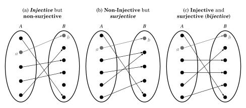
The function mapping on the left is an example of an injective function because it is one-to-one. However, it is not surjective because the range and the codomain are not the same.
- A function is injective if it is one-to-one.
- A function is surjective if it is "onto." That is, the mapping has as the range of the function, where the codomain and the range of the function are the same.
- A function is bijective if it is both surjective and injective.
Again, the above definitions are often very confusing. Again, another image is provided to the right of the bullet points. Along with that, another example is also provided. Let us analyze the function  .
.
Given: , where is constant and .
Prove: function is non-surjective and non-injective.
Notice that the only changing element in the function is . Let us check to see the conditions of this function.
Is it injective? Let  , and solve for . First, divide by .


Then take the square root of  . By definition,
  , so
, so


Notice, however, what we learned from the above manipulation. As a result of solving for , we found that there are two solutions for . However, this resulted in two different values from  . This means that for some individual that gives , there are two different inputs that result in the same value. Because
  when , this is by definition non-injective.
Is it surjective? As a natural consequence of what we learned about inputs, let us determine the range of the function. After all, the only way to determine if something is surjective is to see if the range applies to all real numbers. A good way to determine this is by finding a pattern involving our domains. Let us say we input a negative number for the domain:  . This seemingly trivial exercise tells us that negative numbers give us non-negative numbers for our range. This is huge information! For
  , the function always results
  for our range. For the set , we have elements in that set that have no mappings from the set . As such,
  is the codomain of set . Therefore, this function is non-surjective!

This is an example of an expression which fails the vertical line test.
Tests for equations
The vertical line test
The vertical line test is a systematic test to find out if an equation involving and can serve as a function (with the independent variable and the dependent variable). Simply graph the equation and draw a vertical line through each point of the -axis. If any vertical line ever touches the graph at more than one point, then the equation is not a function; if the line always touches at most one point of the graph, then the equation is a function.
The circle, on the right, is not a function because the vertical line intercepts two points on the graph when  .
.
The horizontal line and the algebraic 1-1 test
Similarly, the horizontal line test, though does not test if an equation is a function, tests if a function is injective (one-to-one). If any horizontal line ever touches the graph at more than one point, then the function is not one-to-one; if the line always touches at most one point on the graph, then the function is one-to-one.
The algebraic 1-1 test is the non-geometric way to see if a function is one-to-one. The basic concept is that:
Assume there is a function . If:
 , and
, and  , then
function is one-to-one.
Here is an example: prove that  is injective.
Since the notation is the notation for a function, the equation is a function. So we only need to prove that it is injective. Let and be the inputs of the function and that . Thus,


So, the result is , proving that the function is injective.
Another example is proving that  is not injective.
Using the same method, one can find that  , which is not . So, the function is not injective.
The following arise as a direct consequence of the definition of functions:
- By definition, for each "input" a function returns only one "output", corresponding to that input. While the same output may correspond to more than one input, one input cannot correspond to more than one output. This is expressed graphically as the vertical line test: a line drawn parallel to the axis of the dependent variable (normally vertical) will intersect the graph of a function only once. However, a line drawn parallel to the axis of the independent variable (normally horizontal) may intersect the graph of a function as many times as it likes. Equivalently, this has an algebraic (or formula-based) interpretation. We can always say if , then , but if we only know that then we can't be sure that .
- Each function has a set of values, the function's domain, which it can accept as input. Perhaps this set is all positive real numbers; perhaps it is the set {pork, mutton, beef}. This set must be implicitly/explicitly defined in the definition of the function. You cannot feed the function an element that isn't in the domain, as the function is not defined for that input element.
- Each function has a set of values, the function's range, which it can output. This may be the set of real numbers. It may be the set of positive integers or even the set {0,1}. This set, too, must be implicitly/explicitly defined in the definition of the function.
Functions are an important foundation of mathematics. This modern interpretation is a result of the hard work of the mathematicians of history. It was not until recently that the definition of the relation was introduced by René Descartes in Geometry (1637). Nearly a century later, the standard notation ( ) was first introduced by Leonhard Euler in Introductio in Analysin Infinitorum and Institutiones Calculi Differentialis. The term function was also a new innovation during Euler's time as well, being introduced Gottfried Wilhelm Leibniz in a 1673 letter "to describe a quantity related to points of a curve, such as a coordinate or curve's slope." Finally, the modern definition of the function being the relation among sets was first introduced in 1908 by Godfrey Harold Hardy where there is a relation between two variables and such that "to some values of at any rate correspond values of ."
Important functions
Polynomials
Polynomial functions are the most common and most convenient functions in the world of calculus. Their frequent appearances and their applications on computer calculations have made them important.
A polynomial in a single indeterminate x can always be written (or rewritten) in the form:

To be more concise, it can also be written in the summation form:

Constant

Two linear functions are shown on the image. One is

and the other is

When  , the polynomial can be rewritten into the following function:
 , where
  is a constant.
The graph of this function is a horizontal line passing the point  .
.
Linear
When  , the polynomial can be rewritten into
 , where
  are constants.
The graph of this function is a straight line passing the point  and
and  , and the slope of this function is
  .
.

This is the graph of a quadratic function.
Quadratic
When  , the polynomial can be rewritten into
 , where
  are constants.
The graph of this function is a parabola, like the trajectory of a basketball thrown into the hoop.
If there are questions about the quadratic formula and other basic polynomial concepts, please review the respective chapters in Algebra.
Trigonometric
Trigonometric functions are also very important because it can connect algebra and geometry. Trigonometric functions are explained in detail here due to its importance and difficulty.
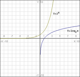
The curve on the left is an exponential function while the curve on the right is a logarithmic one
Exponential and Logarithmic
Exponential and logarithmic functions have a unique identity when calculating the derivatives, so this is a great time to review those functions.
The exponential function is defined as:
 , where is a constant.
while the logarithmic function is defined as:
 , where is a constant.
A special number will be frequently seen in those functions: the Euler's constant, also known as the base of the natural logarithm. Notated as  , it is defined as
  .
.
Signum
The Signum (sign) function is simply defined as

Properties of functions
Sometimes, a lot of function manipulations cannot be achieved without some help from basic properties of functions.
Domain and range
This concept is discussed above.
Growth
Although it seems obvious to spot a function increasing or decreasing, without the help of graphing software, we need a mathematical way to spot whether the function is increasing or decreasing, or else our human minds cannot immediately comprehend the huge amount of information.
Assume a function with inputs  , and that
 ![{\displaystyle x_{1}\in [a,b]}](https://wikimedia.org/api/rest_v1/media/math/render/svg/0f03ee615e7879f20efa45f3c3c6296c14b53995) ,
, ![{\displaystyle x_{2}\in [a,b]}](https://wikimedia.org/api/rest_v1/media/math/render/svg/e93c068e15bd53700224ed82f922c758216ee03e) , and
, and  at all times.
If for all and ,  , then
is increasing in ![{\displaystyle [a,b]}](https://wikimedia.org/api/rest_v1/media/math/render/svg/9c4b788fc5c637e26ee98b45f89a5c08c85f7935)
If for all and ,  , then
is decreasing in
Example: In which intervals is  increasing?
Firstly, the domain is important. Because the denominator cannot be 0, the domain for this function is

In  , the growth of the function is:
Let ![{\displaystyle x_{1},x_{2}\in [-\infty ,-1]}](https://wikimedia.org/api/rest_v1/media/math/render/svg/0cf5c7151b951ae1ff019d7e81b7649743e9a8ac) and
Thus,
and
Thus,

 both
both


and 

So, 
is decreasing in
In 
Let ![{\displaystyle x_{1},x_{2}\in [-1,1]}](https://wikimedia.org/api/rest_v1/media/math/render/svg/8ed87fe12ce57afdf247fb00036ed2503255e93f) and
Thus,
and
Thus,
both
However, the sign of  in cannot be determined. It can only be determined in
  .
.
In 
and
In 


As a result,
is decreasing in and increasing in .
In 
Let ![{\displaystyle x_{1},x_{2}\in [1,\infty ]}](https://wikimedia.org/api/rest_v1/media/math/render/svg/740ee44dae32033ccc8b24018acf55e6c11fa60a) and
Thus,
and
Thus,
both
So, 
is increasing in .
Therefore, the intervals in which the function is increasing are  .
.

After learning derivatives, there will be more ways to determine the growth of a function.
Parity
The properties odd and even are associated with symmetry. While even functions have a symmetry about the -axis, odd functions are symmetric about the origin. In mathematical terms:
A function is even when  A function is odd when
Example: Prove that is an even function.

 is an even function
Manipulating functions
Addition, Subtraction, Multiplication and Division of functions
For two real-valued functions, we can add the functions, multiply the functions,
raised to a power, etc. For example:
- If we add the functions and
 , we obtain
  .
.
- If we subtract from , we obtain
 . We can also write this as
  .
.
- If we multiply the function and the function , we obtain
 . We can also write this as
  .
.
- If we divide the function by the function , we obtain
 .
.
If a math problem wants you to add two functions and , there are two ways that the problem will likely be worded:
- If you are told that , that , that
 and asked about , then you are being asked to add two functions. Your answer would be
  .
.
- If you are told that , that and you are asked about
 , then you are being asked to add two functions. The addition of and is called . Your answer would be
  .
.
Similar statements can be made for subtraction, multiplication and division.
Let and: . Let's add, subtract, multiply and divide.
 ,
,
 ,
,
 ,
,
 .
.
Composition of functions
We begin with a fun (and not too complicated) application of composition of functions before we talk about what composition of functions is.
Example: Dropping a ball
If we drop a ball from a bridge which is 20 meters above the ground, then the height of our ball above the earth is a function of time. The physicists tell us that if we measure time in seconds and distance in meters, then the formula for height in terms of time is  . Suppose we are tracking the ball with a camera and always want the ball to be in the center of our picture. Suppose we have
  The angle will depend upon the height of the ball above the ground and the height above the ground depends upon time. So the angle will depend upon time. This can be written as
  . We replace with what it is equal to. This is the essence of composition.
Composition of functions is another way to combine functions which is different from addition,
subtraction, multiplication or division.
The value of a function depends upon the value of another variable ; however, that variable could be equal to another function , so its value depends on the value of a third variable. If this is the case, then the first variable is a function of the third variable; this function () is called the composition of the other two functions ( and ).
Example: Composing two functions
Let and: . The composition of with is read as either "f composed with g" or "f of g of x."
Let

Then
 .
.
Sometimes a math problem asks you compute  when they want you to compute
  ,
,
Here, is the composition of and and we write  . Note that composition is not commutative:
 , and
, and

- so
 .
.
Composition of functions is very common, mainly because functions themselves are common. For instance, squaring and sine are both functions:


Thus, the expression  is a composition of functions:
|
|

|
|
|

|
(Note that this is not the same as  .)
Since the function sine equals
.)
Since the function sine equals  if
if  ,
,
 .
.
Since the function square equals  if ,
if ,
 .
.
Transformations
Transformations are a type of function manipulation that are very common. They consist of multiplying, dividing, adding or subtracting constants to either the input or the output. Multiplying by a constant is called dilation and adding a constant is called translation. Here are a few examples:
 Dilation
 Translation
 Dilation
 Translation

Examples of horizontal and vertical translations

Examples of horizontal and vertical dilations
Translations and dilations can be either horizontal or vertical. Examples of both vertical and horizontal translations can be seen at right. The red graphs represent functions in their 'original' state, the solid blue graphs have been translated (shifted) horizontally, and the dashed graphs have been translated vertically.
Dilations are demonstrated in a similar fashion. The function
has had its input doubled. One way to think about this is that now any change in the input will be doubled. If I add one to , I add two to the input of , so it will now change twice as quickly. Thus, this is a horizontal dilation by  because the distance to the -axis has been halved. A vertical dilation, such as
is slightly more straightforward. In this case, you double the output of the function. The output represents the distance from the -axis, so in effect, you have made the graph of the function 'taller'. Here are a few basic examples where is any positive constant:
| Original graph
|
|
Rotation about origin
|

|
| Horizontal translation by units left
|

|
Horizontal translation by units right
|

|
| Horizontal dilation by a factor of
|

|
Vertical dilation by a factor of
|

|
| Vertical translation by units down
|

|
Vertical translation by units up
|

|
| Reflection about -axis
|

|
Reflection about -axis
|

|
Inverse functions
We call  the inverse function of if, for all :

A function has an inverse function if and only if is one-to-one. For example, the inverse of  is
is  . The function has no inverse because it is not injective. Similarly, the inverse functions of trigonometric functions have to undergo transformations and limitations to be considered as valid functions.
Notation
The inverse function of is denoted as  . Thus, is defined as the function that follows this rule

To determine when given a function , substitute for and substitute for . Then solve for , provided that it is also a function.
Example: Given  , find .
Substitute for and substitute for . Then solve for :
![{\displaystyle \Leftrightarrow x=2[f^{-1}(x)]-7}](https://wikimedia.org/api/rest_v1/media/math/render/svg/d823629e07ebfdf4e31604db723251807f12fd12)
![{\displaystyle \Leftrightarrow x+7=2[f^{-1}(x)]}](https://wikimedia.org/api/rest_v1/media/math/render/svg/5ef00069307c01d1d32178da59bf982da21648af)

To check your work, confirm that  :
:


If isn't one-to-one, then, as we said before, it doesn't have an inverse. Then this method will fail.
Example: Given  , find .
Substitute for and substitute for . Then solve for :


Since there are two possibilities for , it's not a function. Thus doesn't have an inverse. Of course, we could also have found this out from the graph by applying the Horizontal Line Test. It's useful, though, to have lots of ways to solve a problem, since in a specific case some of them might be very difficult while others might be easy. For example, we might only know an algebraic expression for but not a graph.
Resources
Licensing
Content obtained and/or adapted from:


