Display of Numerical Data
Bar graphs
A bar chart or bar graph is a chart or graph that presents categorical data with rectangular bars with heights or lengths proportional to the values that they represent. The bars can be plotted vertically or horizontally. A vertical bar chart is sometimes called a column chart.
Usage
Bar graphs/charts provide a visual presentation of categorical data. Categorical data is a grouping of data into discrete groups, such as months of the year, age group, shoe sizes, and animals. These categories are usually qualitative. In a column (vertical) bar chart, categories appear along the horizontal axis and the height of the bar corresponds to the value of each category.
Bar charts have a discrete domain of categories, and are usually scaled so that all the data can fit on the chart. When there is no natural ordering of the categories being compared, bars on the chart may be arranged in any order. Bar charts arranged from highest to lowest incidence are called Pareto charts.
Grouped (clustered) and stacked
Bar graphs can also be used for more complex comparisons of data with grouped (or "clustered") bar charts, and stacked bar charts.
In grouped (clustered) bar charts, for each categorical group there are two or more bars color-coded to represent a particular grouping. For example, a business owner with two stores might make a grouped bar chart with different colored bars to represent each store: the horizontal axis would show the months of the year and the vertical axis would show revenue.
Alternatively, a stacked bar chart stacks bars on top of each other so that the height of the resulting stack shows the combined result. Stacked bar charts are not suited to data sets having both positive and negative values.
Grouped bar charts usually present the information in the same order in each grouping. Stacked bar charts present the information in the same sequence on each bar.

A vertical stacked bar chart with positive values

A vertical stacked bar chart with negative values

A horizontal stacked bar chart

A vertical, grouped (clustered) 3D bar chart


Histogram
A histogram is an approximate representation of the distribution of numerical data. It was first introduced by Karl Pearson. To construct a histogram, the first step is to "bin" (or "bucket") the range of values—that is, divide the entire range of values into a series of intervals—and then count how many values fall into each interval. The bins are usually specified as consecutive, non-overlapping intervals of a variable. The bins (intervals) must be adjacent and are often (but not required to be) of equal size.
If the bins are of equal size, a rectangle is erected over the bin with height proportional to the frequency—the number of cases in each bin. A histogram may also be normalized to display "relative" frequencies. It then shows the proportion of cases that fall into each of several categories, with the sum of the heights equaling 1.
However, bins need not be of equal width; in that case, the erected rectangle is defined to have its area proportional to the frequency of cases in the bin. The vertical axis is then not the frequency but frequency density—the number of cases per unit of the variable on the horizontal axis. Examples of variable bin width are displayed on Census bureau data below.
As the adjacent bins leave no gaps, the rectangles of a histogram touch each other to indicate that the original variable is continuous.
Histograms give a rough sense of the density of the underlying distribution of the data, and often for density estimation: estimating the probability density function of the underlying variable. The total area of a histogram used for probability density is always normalized to 1. If the length of the intervals on the x-axis are all 1, then a histogram is identical to a relative frequency plot.
A histogram can be thought of as a simplistic kernel density estimation, which uses a kernel to smooth frequencies over the bins. This yields a smoother probability density function, which will in general more accurately reflect distribution of the underlying variable. The density estimate could be plotted as an alternative to the histogram, and is usually drawn as a curve rather than a set of boxes. Histograms are nevertheless preferred in applications, when their statistical properties need to be modeled. The correlated variation of a kernel density estimate is very difficult to describe mathematically, while it is simple for a histogram where each bin varies independently.
An alternative to kernel density estimation is the average shifted histogram, which is fast to compute and gives a smooth curve estimate of the density without using kernels.
The histogram is one of the seven basic tools of quality control.
Histograms are sometimes confused with bar charts. A histogram is used for continuous data, where the bins represent ranges of data, while a bar chart is a plot of categorical variables. Some authors recommend that bar charts have gaps between the rectangles to clarify the distinction.
Examples
This is the data for the histogram to the right, using 500 items:
| Bin/Interval | Count/Frequency |
|---|---|
| −3.5 to −2.51 | 9 |
| −2.5 to −1.51 | 32 |
| −1.5 to −0.51 | 109 |
| −0.5 to 0.49 | 180 |
| 0.5 to 1.49 | 132 |
| 1.5 to 2.49 | 34 |
| 2.5 to 3.49 | 4 |
The words used to describe the patterns in a histogram are: "symmetric", "skewed left" or "right", "unimodal", "bimodal" or "multimodal".

Symmetric, unimodal

Skewed right
Skewed left
Bimodal
Multimodal
Symmetric


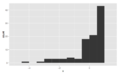
It is a good idea to plot the data using several different bin widths to learn more about it. Here is an example on tips given in a restaurant.
- Tips-histogram1.png
Tips using a $1 bin width, skewed right, unimodal
- Tips-histogram2.png
Tips using a 10c bin width, still skewed right, multimodal with modes at $ and 50c amounts, indicates rounding, also some outliers
The U.S. Census Bureau found that there were 124 million people who work outside of their homes. Using their data on the time occupied by travel to work, the table below shows the absolute number of people who responded with travel times "at least 30 but less than 35 minutes" is higher than the numbers for the categories above and below it. This is likely due to people rounding their reported journey time. The problem of reporting values as somewhat arbitrarily rounded numbers is a common phenomenon when collecting data from people.
Data by absolute numbers Interval Width Quantity Quantity/width 0 5 4180 836 5 5 13687 2737 10 5 18618 3723 15 5 19634 3926 20 5 17981 3596 25 5 7190 1438 30 5 16369 3273 35 5 3212 642 40 5 4122 824 45 15 9200 613 60 30 6461 215 90 60 3435 57
This histogram shows the number of cases per unit interval as the height of each block, so that the area of each block is equal to the number of people in the survey who fall into its category. The area under the curve represents the total number of cases (124 million). This type of histogram shows absolute numbers, with Q in thousands.
Data by proportion Interval Width Quantity (Q) Q/total/width 0 5 4180 0.0067 5 5 13687 0.0221 10 5 18618 0.0300 15 5 19634 0.0316 20 5 17981 0.0290 25 5 7190 0.0116 30 5 16369 0.0264 35 5 3212 0.0052 40 5 4122 0.0066 45 15 9200 0.0049 60 30 6461 0.0017 90 60 3435 0.0005
This histogram differs from the first only in the vertical scale. The area of each block is the fraction of the total that each category represents, and the total area of all the bars is equal to 1 (the fraction meaning "all"). The curve displayed is a simple density estimate. This version shows proportions, and is also known as a unit area histogram.
In other words, a histogram represents a frequency distribution by means of rectangles whose widths represent class intervals and whose areas are proportional to the corresponding frequencies: the height of each is the average frequency density for the interval. The intervals are placed together in order to show that the data represented by the histogram, while exclusive, is also contiguous. (E.g., in a histogram it is possible to have two connecting intervals of 10.5–20.5 and 20.5–33.5, but not two connecting intervals of 10.5–20.5 and 22.5–32.5. Empty intervals are represented as empty and not skipped.)
Dot plots
A dot chart or dot plot is a statistical chart consisting of data points plotted on a fairly simple scale, typically using filled in circles. There are two common, yet very different, versions of the dot chart. The first has been used in hand-drawn (pre-computer era) graphs to depict distributions going back to 1884. The other version is described by William S. Cleveland as an alternative to the bar chart, in which dots are used to depict the quantitative values (e.g. counts) associated with categorical variables.
Of a distribution
The dot plot as a representation of a distribution consists of group of data points plotted on a simple scale. Dot plots are used for continuous, quantitative, univariate data. Data points may be labelled if there are few of them.
Dot plots are one of the simplest statistical plots, and are suitable for small to moderate sized data sets. They are useful for highlighting clusters and gaps, as well as outliers. Their other advantage is the conservation of numerical information. When dealing with larger data sets (around 20–30 or more data points) the related stemplot, box plot or histogram may be more efficient, as dot plots may become too cluttered after this point. Dot plots may be distinguished from histograms in that dots are not spaced uniformly along the horizontal axis.
Although the plot appears to be simple, its computation and the statistical theory underlying it are not simple. The algorithm for computing a dot plot is closely related to kernel density estimation. The size chosen for the dots affects the appearance of the plot. Choice of dot size is equivalent to choosing the bandwidth for a kernel density estimate.
In the R programming language this type of plot is also referred to as a stripchart or stripplot.
Cleveland dot plots
Dot plot may also refer to plots of points that each belong to one of several categories. They are an alternative to bar charts or pie charts, and look somewhat like a horizontal bar chart where the bars are replaced by a dots at the values associated with each category. Compared to (vertical) bar charts and pie charts, Cleveland argues that dot plots allow more accurate interpretation of the graph by readers by making the labels easier to read, reducing non-data ink (or graph clutter) and supporting table look-up.
Box plot
In descriptive statistics, a box plot or boxplot is a method for graphically demonstrating the locality, spread and skewness groups of numerical data through their quartiles. In addition to the box on a box plot, there can be lines (which are called whiskers) extending from the box indicating variability outside the upper and lower quartiles, thus, the plot is also termed as the box-and-whisker plot and the box-and-whisker diagram. Outliers that differ significantly from the rest of the dataset may be plotted as individual points beyond the whiskers on the box-plot. Box plots are non-parametric: they display variation in samples of a statistical population without making any assumptions of the underlying statistical distribution (though Tukey's boxplot assumes symmetry for the whiskers and normality for their length). The spacings in each subsection of the box-plot indicate the degree of dispersion (spread) and skewness of the data, which are usually described using the five-number summary. In addition, the box-plot allows one to visually estimate various L-estimators, notably the interquartile range, midhinge, range, mid-range, and trimean. Box plots can be drawn either horizontally or vertically.
History
The range-bar method was first introduced by Mary Eleanor Spear in her book "Charting Statistics" in 1952 and again in her book "Practical Charting Techniques" in 1969. The box-and-whisker plot was first introduced in 1970 by John Tukey, who later published on the subject in his book "Exploratory Data Analysis" in 1977.
Elements
A boxplot is a standardized way of displaying the dataset based on the five-number summary: the minimum, the maximum, the sample median, and the first and third quartiles.
- Minimum (Q0 or 0th percentile): the lowest data point in the data set excluding any outliers
- Maximum (Q4 or 100th percentile): the highest data point in the data set excluding any outliers
- Median (Q2 or 50th percentile): the middle value in the data set
- First quartile (Q1 or 25th percentile): also known as the lower quartile qn(0.25), it is the median of the lower half of the dataset.
- Third quartile (Q3 or 75th percentile): also known as the upper quartile qn(0.75), it is the median of the upper half of the dataset.
In addition to the minimum and maximum values used to construct a box-plot, another important element that can also be employed to obtain a box-plot is the interquartile range (IQR), as denoted below:
- Interquartile range (IQR) : the distance between the upper and lower quartiles

A box-plot usually includes two parts, a box and a set of whiskers as shown in Figure 2. The lowest point on the box-plot (i.e. the boundary of the lower whisker) is the minimum value of the data set and the highest point (i.e. the boundary of the upper whisker) is the maximum value of the data set (excluding any outliers). The box is drawn from Q1 to Q3 with a horizontal line drawn in the middle to denote the median.
The same data set can also be made into a box-plot through a different approach as shown in Figure 3. This time the boundaries of the whiskers are found within the 1.5 IQR value. From above the upper quartile (Q3), a distance of 1.5 times the IQR is measured out and a whisker is drawn up to the largest observed data point from the dataset that falls within this distance. Similarly, a distance of 1.5 times the IQR is measured out below the lower quartile (Q1) and a whisker is drawn down to the lowest observed data point from the dataset that falls within this distance. All other observed data points outside the boundary of the whiskers are plotted as outliers. The outliers can be plotted on the box-plot as a dot, a small circle, a star, etc..
However, the whiskers can stand for several other things, such as:
- The minimum and the maximum value of the data set (as shown in Figure 2)
- One standard deviation above and below the mean of the data set
- The 9th percentile and the 91st percentile of the data set
- The 2nd percentile and the 98th percentile of the data set
Rarely, box-plot can be plotted without the whiskers.
Some box plots include an additional character to represent the mean of the data.
The unusual percentiles 2%, 9%, 91%, 98% are sometimes used for whisker cross-hatches and whisker ends to depict the seven-number summary. If the data are normally distributed, the locations of the seven marks on the box plot will be equally spaced. On some box plots, a cross-hatch is placed before the end of each whisker.
Because of this variability, it is appropriate to describe the convention that is being used for the whiskers and outliers in the caption of the box-plot.
Variations
Since the mathematician John W. Tukey first popularized this type of visual data display in 1969, several variations on the classical box plot have been developed, and the two most commonly found variations are the variable width box plots and the notched box plots shown in Figure 4.
Variable width box plots illustrate the size of each group whose data is being plotted by making the width of the box proportional to the size of the group. A popular convention is to make the box width proportional to the square root of the size of the group.
Notched box plots apply a "notch" or narrowing of the box around the median. Notches are useful in offering a rough guide of the significance of the difference of medians; if the notches of two boxes do not overlap, this will provide evidence of a statistically significant difference between the medians. The width of the notches is proportional to the interquartile range (IQR) of the sample and is inversely proportional to the square root of the size of the sample. However, there is a uncertainty about the most appropriate multiplier (as this may vary depending on the similarity of the variances of the samples).
One convention for obtaining the boundaries of these notches is to use a distance of around the median.

Adjusted box plots are intended to describe skew distributions, and they rely on the medcouple statistic of skewness. For a medcouple value of MC, the lengths of the upper and lower whiskers on the box-plot are respectively defined to be:

For a symmetrical data distribution, the medcouple will be zero, and this reduces the adjusted box-plot to the Tukey's box-plot with equal whisker lengths of Failed to parse (MathML with SVG or PNG fallback (recommended for modern browsers and accessibility tools): Invalid response ("Math extension cannot connect to Restbase.") from server "https://wikimedia.org/api/rest_v1/":): {\displaystyle 1.5 \text{ IQR}} for both whiskers.
Other kinds of box plots, such as the violin plots and the bean plots can show the difference between single-modal and multimodal distributions, which cannot be observed from the original classical box-plot.
Examples
Example without outliers
A series of hourly temperatures were measured throughout the day in degrees Fahrenheit. The recorded values are listed in order as follows (°F): 57, 57, 57, 58, 63, 66, 66, 67, 67, 68, 69, 70, 70, 70, 70, 72, 73, 75, 75, 76, 76, 78, 79, 81.
A box plot of the data set can be generated by first calculating five relevant values of this data set: minimum, maximum, median (Q2), first quartile (Q1), and third quartile (Q3).
The minimum is the smallest number of the data set. In this case, the minimum recorded day temperature is 57 °F.
The maximum is the largest number of the data set. In this case, the maximum recorded day temperature is 81 °F.
The median is the "middle" number of the ordered data set. This means that there are exactly 50% of the elements is less than the median and 50% of the elements is greater than the median. The median of this ordered data set is 70 °F.
The first quartile value (Q1 or 25th percentile) is the number that marks one quarter of the ordered data set. In other words, there are exactly 25% of the elements that are less than the first quartile and exactly 75% of the elements that are greater than it. The first quartile value can be easily determined by finding the "middle" number between the minimum and the median. For the hourly temperatures, the "middle" number found between 57 °F and 70 °F is 66 °F.
The third quartile value (Q3 or 75th percentile) is the number that marks three quarters of the ordered data set. In other words, there are exactly 75% of the elements that are less than the third quartile and 25% of the elements that are greater than it. The third quartile value can be easily obtained by finding the "middle" number between the median and the maximum. For the hourly temperatures, the "middle" number between 70 °F and 81 °F is 75 °F.
The interquartile range, or IQR, can be calculated by subtracting the first quartile value (Q1) from the third quartile value (Q3):
- Failed to parse (MathML with SVG or PNG fallback (recommended for modern browsers and accessibility tools): Invalid response ("Math extension cannot connect to Restbase.") from server "https://wikimedia.org/api/rest_v1/":): {\displaystyle \text{IQR} = Q_3 - Q_1=75^\circ F-66^\circ F=9^\circ F.}
Hence, Failed to parse (MathML with SVG or PNG fallback (recommended for modern browsers and accessibility tools): Invalid response ("Math extension cannot connect to Restbase.") from server "https://wikimedia.org/api/rest_v1/":): {\displaystyle 1.5 \text{IQR}=1.5 \cdot 9^\circ F=13.5 ^\circ F.}
1.5 IQR above the third quartile is:
- Failed to parse (MathML with SVG or PNG fallback (recommended for modern browsers and accessibility tools): Invalid response ("Math extension cannot connect to Restbase.") from server "https://wikimedia.org/api/rest_v1/":): {\displaystyle Q3+1.5\text{ IQR}=75^\circ F+13.5^\circ F=88.5^\circ F.}
1.5 IQR below the first quartile is:
- Failed to parse (MathML with SVG or PNG fallback (recommended for modern browsers and accessibility tools): Invalid response ("Math extension cannot connect to Restbase.") from server "https://wikimedia.org/api/rest_v1/":): {\displaystyle Q_1-1.5\text{ IQR}=66^\circ F-13.5^\circ F=52.5^\circ F.}
The upper whisker boundary of the box-plot is the largest data value that is within 1.5 IQR above the third quartile. Here, 1.5 IQR above the third quartile is 88.5 °F and the maximum is 81 °F. Therefore, the upper whisker is drawn at the value of the maximum, which is 81 °F.
Similarly, the lower whisker boundary of the box plot is the smallest data value that is within 1.5 IQR below the first quartile. Here, 1.5 IQR below the first quartile is 52.5 °F and the minimum is 57 °F. Therefore, the lower whisker is drawn at the value of the minimum, which is 57 °F.
Example with outliers
Above is an example without outliers. Here is a followup example for generating box-plot with outliers:
The ordered set for the recorded temperatures is (°F): 52, 57, 57, 58, 63, 66, 66, 67, 67, 68, 69, 70, 70, 70, 70, 72, 73, 75, 75, 76, 76, 78, 79, 89.
In this example, only the first and the last number are changed. The median, third quartile, and first quartile remain the same.
In this case, the maximum value in this data set is 89 °F, and 1.5 IQR above the third quartile is 88.5 °F. The maximum is greater than 1.5 IQR plus the third quartile, so the maximum is an outlier. Therefore, the upper whisker is drawn at the greatest value smaller than 1.5 IQR above the third quartile, which is 79 °F.
Similarly, the minimum value in this data set is 52 °F, and 1.5 IQR below the first quartile is 52.5 °F. The minimum is smaller than 1.5 IQR minus the first quartile, so the minimum is also an outlier. Therefore, the lower whisker is drawn at the smallest value greater than 1.5 IQR below the first quartile, which is 57 °F.
In the case of large datasets
An additional example for obtaining box-plot from a data set containing a large number of data points is:
General equation to compute empirical quantiles
- Failed to parse (MathML with SVG or PNG fallback (recommended for modern browsers and accessibility tools): Invalid response ("Math extension cannot connect to Restbase.") from server "https://wikimedia.org/api/rest_v1/":): {\displaystyle q_n(p) = x_{(k)} + \alpha(x_{(k+1)} - x_{(k)})}
- Failed to parse (MathML with SVG or PNG fallback (recommended for modern browsers and accessibility tools): Invalid response ("Math extension cannot connect to Restbase.") from server "https://wikimedia.org/api/rest_v1/":): {\displaystyle \text{with } k = [p(n+1)] \text{ and } \alpha = p(n+1) - k}
- Here Failed to parse (MathML with SVG or PNG fallback (recommended for modern browsers and accessibility tools): Invalid response ("Math extension cannot connect to Restbase.") from server "https://wikimedia.org/api/rest_v1/":): {\displaystyle x_{(k)}} stands for the general ordering of the data points (i.e. if Failed to parse (MathML with SVG or PNG fallback (recommended for modern browsers and accessibility tools): Invalid response ("Math extension cannot connect to Restbase.") from server "https://wikimedia.org/api/rest_v1/":): {\displaystyle i<k} , then Failed to parse (MathML with SVG or PNG fallback (recommended for modern browsers and accessibility tools): Invalid response ("Math extension cannot connect to Restbase.") from server "https://wikimedia.org/api/rest_v1/":): {\displaystyle x_{(i)} < x_{(k)}} )
Using the above example that has 24 data points (n = 24), one can calculate the median, first and third quartile either mathematically or visually.
Median : Failed to parse (MathML with SVG or PNG fallback (recommended for modern browsers and accessibility tools): Invalid response ("Math extension cannot connect to Restbase.") from server "https://wikimedia.org/api/rest_v1/":): {\displaystyle q_n(0.5) = x_{(12)} + (0.5\cdot25-12)\cdot(x_{(13)}-x_{(12)}) = 70+(0.5\cdot25-12)\cdot(70-70) = 70^\circ F}
First quartile : Failed to parse (MathML with SVG or PNG fallback (recommended for modern browsers and accessibility tools): Invalid response ("Math extension cannot connect to Restbase.") from server "https://wikimedia.org/api/rest_v1/":): {\displaystyle q_n(0.25) = x_{(6)} + (0.25\cdot25-6)\cdot(x_{(7)}-x_{(6)}) = 66 +(0.25\cdot25 - 6)\cdot(66-66) = 66^\circ F}
Third quartile : Failed to parse (MathML with SVG or PNG fallback (recommended for modern browsers and accessibility tools): Invalid response ("Math extension cannot connect to Restbase.") from server "https://wikimedia.org/api/rest_v1/":): {\displaystyle q_n(0.75) = x_{(18)} + (0.75\cdot25-18)\cdot(x_{(19)}-x_{(18)}) =75 + (0.75\cdot25-18)\cdot(75-75) = 75^\circ F}
Visualization
Although box plots may seem more primitive than histograms or kernel density estimates, they do have a number of advantages. First, the box plot enables statisticians to do a quick graphical examination on one or more data sets. Box-plots also take up less space and are therefore particularly useful for comparing distributions between several groups or sets of data in parallel (see Figure 1 for an example). Lastly, the overall structure of histograms and kernel density estimate can be strongly influenced by the choice of number and width of bins techniques and the choice of bandwidth, respectively.
Although looking at a statistical distribution is more common than looking at a box plot, it can be useful to compare the box plot against the probability density function (theoretical histogram) for a normal N(0,σ2) distribution and observe their characteristics directly (as shown in Figure 7).
Mean absolute deviation
The average absolute deviation (AAD) of a data set is the average of the absolute deviations from a central point. It is a summary statistic of statistical dispersion or variability. In the general form, the central point can be a mean, median, mode, or the result of any other measure of central tendency or any reference value related to the given data set. AAD includes the mean absolute deviation and the median absolute deviation (both abbreviated as MAD).
Measures of dispersion
Several measures of statistical dispersion are defined in terms of the absolute deviation. The term "average absolute deviation" does not uniquely identify a measure of statistical dispersion, as there are several measures that can be used to measure absolute deviations, and there are several measures of central tendency that can be used as well. Thus, to uniquely identify the absolute deviation it is necessary to specify both the measure of deviation and the measure of central tendency. Unfortunately, the statistical literature has not yet adopted a standard notation, as both the mean absolute deviation around the mean and the median absolute deviation around the median have been denoted by their initials "MAD" in the literature, which may lead to confusion, since in general, they may have values considerably different from each other.
Mean absolute deviation around a central point
The mean absolute deviation of a set {x1, x2, ..., xn} is
- Failed to parse (MathML with SVG or PNG fallback (recommended for modern browsers and accessibility tools): Invalid response ("Math extension cannot connect to Restbase.") from server "https://wikimedia.org/api/rest_v1/":): {\displaystyle \frac{1}{n}\sum_{i=1}^n |x_i-m(X)|.}
The choice of measure of central tendency, Failed to parse (MathML with SVG or PNG fallback (recommended for modern browsers and accessibility tools): Invalid response ("Math extension cannot connect to Restbase.") from server "https://wikimedia.org/api/rest_v1/":): {\displaystyle m(X)} , has a marked effect on the value of the mean deviation. For example, for the data set {2, 2, 3, 4, 14}:
| Measure of central tendency Failed to parse (MathML with SVG or PNG fallback (recommended for modern browsers and accessibility tools): Invalid response ("Math extension cannot connect to Restbase.") from server "https://wikimedia.org/api/rest_v1/":): {\displaystyle m(X)} | Mean absolute deviation |
|---|---|
| Mean = 5 | Failed to parse (MathML with SVG or PNG fallback (recommended for modern browsers and accessibility tools): Invalid response ("Math extension cannot connect to Restbase.") from server "https://wikimedia.org/api/rest_v1/":): {\displaystyle \frac{|2 - 5| + |2 - 5| + |3 - 5| + |4 - 5| + |14 - 5|}{5} = 3.6} |
| Median = 3 | Failed to parse (MathML with SVG or PNG fallback (recommended for modern browsers and accessibility tools): Invalid response ("Math extension cannot connect to Restbase.") from server "https://wikimedia.org/api/rest_v1/":): {\displaystyle \frac{|2 - 3| + |2 - 3| + |3 - 3| + |4 - 3| + |14 - 3|}{5} = 2.8} |
| Mode = 2 | Failed to parse (MathML with SVG or PNG fallback (recommended for modern browsers and accessibility tools): Invalid response ("Math extension cannot connect to Restbase.") from server "https://wikimedia.org/api/rest_v1/":): {\displaystyle \frac{|2 - 2| + |2 - 2| + |3 - 2| + |4 - 2| + |14 - 2|}{5} = 3.0} |
The mean absolute deviation from the median is less than or equal to the mean absolute deviation from the mean. In fact, the mean absolute deviation from the median is always less than or equal to the mean absolute deviation from any other fixed number.
The mean absolute deviation from the mean is less than or equal to the standard deviation; one way of proving this relies on Jensen's inequality.
Proof Jensen's inequality is Failed to parse (MathML with SVG or PNG fallback (recommended for modern browsers and accessibility tools): Invalid response ("Math extension cannot connect to Restbase.") from server "https://wikimedia.org/api/rest_v1/":): {\displaystyle \varphi\left(\mathbb{E}[Y]\right) \leq \mathbb{E}\left[\varphi(Y)\right]} ,where φ is a convex function, this implies for Failed to parse (MathML with SVG or PNG fallback (recommended for modern browsers and accessibility tools): Invalid response ("Math extension cannot connect to Restbase.") from server "https://wikimedia.org/api/rest_v1/":): {\displaystyle Y = \vert X-\mu\vert } that: - Failed to parse (MathML with SVG or PNG fallback (recommended for modern browsers and accessibility tools): Invalid response ("Math extension cannot connect to Restbase.") from server "https://wikimedia.org/api/rest_v1/":): {\displaystyle \mathbb{E}\left( |X -\mu \right|)^{2}\leq\mathbb{E}\left(|X-\mu|^2 \right)}
- Failed to parse (MathML with SVG or PNG fallback (recommended for modern browsers and accessibility tools): Invalid response ("Math extension cannot connect to Restbase.") from server "https://wikimedia.org/api/rest_v1/":): {\displaystyle \mathbb{E}\left( |X -\mu \right|)^{2}\leq \operatorname{Var}(X)}
Since both sides are positive, and the square root is a monotonically increasing function in the positive domain:
- Failed to parse (MathML with SVG or PNG fallback (recommended for modern browsers and accessibility tools): Invalid response ("Math extension cannot connect to Restbase.") from server "https://wikimedia.org/api/rest_v1/":): {\displaystyle \mathbb{E}\left(|X -\mu \right|)\leq \sqrt{\operatorname{Var}(X)}}
For a general case of this statement, see Hölder's inequality.
For the normal distribution, the ratio of mean absolute deviation to standard deviation is Failed to parse (MathML with SVG or PNG fallback (recommended for modern browsers and accessibility tools): Invalid response ("Math extension cannot connect to Restbase.") from server "https://wikimedia.org/api/rest_v1/":): {\displaystyle \sqrt{2/\pi} = 0.79788456\ldots} . Thus if X is a normally distributed random variable with expected value 0 then, see Geary (1935):
- Failed to parse (MathML with SVG or PNG fallback (recommended for modern browsers and accessibility tools): Invalid response ("Math extension cannot connect to Restbase.") from server "https://wikimedia.org/api/rest_v1/":): {\displaystyle w=\frac{ E|X| }{ \sqrt{E(X^2)} } = \sqrt{\frac{2}{\pi}}. }
In other words, for a normal distribution, mean absolute deviation is about 0.8 times the standard deviation. However, in-sample measurements deliver values of the ratio of mean average deviation / standard deviation for a given Gaussian sample n with the following bounds: Failed to parse (MathML with SVG or PNG fallback (recommended for modern browsers and accessibility tools): Invalid response ("Math extension cannot connect to Restbase.") from server "https://wikimedia.org/api/rest_v1/":): {\displaystyle w_n \in [0,1] } , with a bias for small n.
Mean absolute deviation around the mean
The mean absolute deviation (MAD), also referred to as the "mean deviation" or sometimes "average absolute deviation", is the mean of the data's absolute deviations around the data's mean: the average (absolute) distance from the mean. "Average absolute deviation" can refer to either this usage, or to the general form with respect to a specified central point (see above).
MAD has been proposed to be used in place of standard deviation since it corresponds better to real life. Because the MAD is a simpler measure of variability than the standard deviation, it can be useful in school teaching.
This method's forecast accuracy is very closely related to the mean squared error (MSE) method which is just the average squared error of the forecasts. Although these methods are very closely related, MAD is more commonly used because it is both easier to compute (avoiding the need for squaring) and easier to understand.
Mean absolute deviation around the median
The median absolute deviation (MAD median) is the median of the absolute deviation from the median. It is a robust estimator of dispersion.
The MAD median offers a direct measure of the scale of a random variable around its median
- Failed to parse (MathML with SVG or PNG fallback (recommended for modern browsers and accessibility tools): Invalid response ("Math extension cannot connect to Restbase.") from server "https://wikimedia.org/api/rest_v1/":): {\displaystyle D_\text{med} = E|X-\text{median}| }
This is the maximum likelihood estimator of the scale parameter Failed to parse (MathML with SVG or PNG fallback (recommended for modern browsers and accessibility tools): Invalid response ("Math extension cannot connect to Restbase.") from server "https://wikimedia.org/api/rest_v1/":): {\displaystyle b} of the Laplace distribution. For the normal distribution we have Failed to parse (MathML with SVG or PNG fallback (recommended for modern browsers and accessibility tools): Invalid response ("Math extension cannot connect to Restbase.") from server "https://wikimedia.org/api/rest_v1/":): {\displaystyle D_\text{mean} = \sigma \sqrt{2/\pi} \approx 0.797884 \sigma } . Since the median minimizes the average absolute distance, we have Failed to parse (MathML with SVG or PNG fallback (recommended for modern browsers and accessibility tools): Invalid response ("Math extension cannot connect to Restbase.") from server "https://wikimedia.org/api/rest_v1/":): {\displaystyle D_\text{med} \le D_\text{mean}} and Failed to parse (MathML with SVG or PNG fallback (recommended for modern browsers and accessibility tools): Invalid response ("Math extension cannot connect to Restbase.") from server "https://wikimedia.org/api/rest_v1/":): {\displaystyle D_\text{med} =\operatorname{erf}^{-1}(1/2) \sigma \approx 0.67449 \sigma} .
By using the general dispersion function, Habib (2011) defined MAD about median as
- Failed to parse (MathML with SVG or PNG fallback (recommended for modern browsers and accessibility tools): Invalid response ("Math extension cannot connect to Restbase.") from server "https://wikimedia.org/api/rest_v1/":): {\displaystyle D_\text{med} = E|X-\text{median}|=2\operatorname{Cov}(X,I_O) }
where the indicator function is
- Failed to parse (MathML with SVG or PNG fallback (recommended for modern browsers and accessibility tools): Invalid response ("Math extension cannot connect to Restbase.") from server "https://wikimedia.org/api/rest_v1/":): {\displaystyle \mathbf{I}_O := \begin{cases} 1 &\text{if } x > \text{median}, \\ 0 &\text{otherwise}. \end{cases} }
This representation allows for obtaining MAD median correlation coefficients.
For the example {2, 2, 3, 4, 14}: 3 is the median, so the absolute deviations from the median are {1, 1, 0, 1, 11} (reordered as {0, 1, 1, 1, 11}) with a median of 1, in this case unaffected by the value of the outlier 14, so the median absolute deviation (also called MAD) is 1.
Maximum absolute deviation
The maximum absolute deviation around an arbitrary point is the maximum of the absolute deviations of a sample from that point. While not strictly a measure of central tendency, the maximum absolute deviation can be found using the formula for the average absolute deviation as above with Failed to parse (MathML with SVG or PNG fallback (recommended for modern browsers and accessibility tools): Invalid response ("Math extension cannot connect to Restbase.") from server "https://wikimedia.org/api/rest_v1/":): {\displaystyle m(X)=\max(X)} , where Failed to parse (MathML with SVG or PNG fallback (recommended for modern browsers and accessibility tools): Invalid response ("Math extension cannot connect to Restbase.") from server "https://wikimedia.org/api/rest_v1/":): {\displaystyle \max(X)} is the sample maximum.
Minimization
The measures of statistical dispersion derived from absolute deviation characterize various measures of central tendency as minimizing dispersion: The median is the measure of central tendency most associated with the absolute deviation. Some location parameters can be compared as follows:
- L2 norm statistics: the mean minimizes the mean squared error
- L1 norm statistics: the median minimizes average absolute deviation,
- L∞ norm statistics: the mid-range minimizes the maximum absolute deviation
- trimmed L∞ norm statistics: for example, the midhinge (average of first and third quartiles) which minimizes the median absolute deviation of the whole distribution, also minimizes the maximum absolute deviation of the distribution after the top and bottom 25% have been trimmed off.
Estimation
The mean absolute deviation of a sample is a biased estimator of the mean absolute deviation of the population. In order for the absolute deviation to be an unbiased estimator, the expected value (average) of all the sample absolute deviations must equal the population absolute deviation. However, it does not. For the population 1,2,3 both the population absolute deviation about the median and the population absolute deviation about the mean are 2/3. The average of all the sample absolute deviations about the mean of size 3 that can be drawn from the population is 44/81, while the average of all the sample absolute deviations about the median is 4/9. Therefore, the absolute deviation is a biased estimator.
However, this argument is based on the notion of mean-unbiasedness. Each measure of location has its own form of unbiasedness (see entry on biased estimator). The relevant form of unbiasedness here is median unbiasedness.
Licensing
Content obtained and/or adapted from:
- Bar chart, Wikipedia under a CC BY-SA license
- Dot plot (statistics), Wikipedia under a CC BY-SA license
- Histogram, Wikipedia under a CC BY-SA license
- Box plot, Wikipedia under a CC BY-SA license
- Average absolute deviation, Wikipedia under a CC BY-SA license